 Options are the simplest non-trivial financial derivatives around. They are part of the curriculum of every university course on Finance for a good reason: They are everywhere! They are traded on regulated exchanges around the world, change hands over the counter between … consenting adults, enhance or "infect" all sorts of contracts as "embedded options", constitute the main ingredient of insurance policies. In their pure form, their annual volume on U.S. Equity Option exchanges alone exceeds 4 billion contracts!
This is the first of a series of articles that will show you how to compute the fair value of options within Excel without using expensive third party software.
Options come in all sorts and flavors but their simplest type – the European Option – can be simply defined as follows:
A European Call (Put) Option on a non-dividend-paying underlying tradable asset S is a contract between two counterparties A and B that grants A the right – but not the obligation – to buy (sell) from (to) B N units of S at some future time T - referred as expiry - for a fixed price K - referred as strike.
Typically the underlying S is some stock XYZ traded in the country, the currency of which is the same as the denomination currency of the strike K.
In that case the N "units" of S are simply N shares of the stock XYZ and are specified in the option contract. For simplicity we will assume N = 1 below.
For example, the underlying S can be the Microsoft stock, the shares of which are traded in Nasdac in the US under the ticker MSFT with a current price around $94. A European Call Option on one MSFT share (N = 1) with expiry T = 31 Jan 2019 and strike K = $96 grants its holder (counterparty A) the right to buy one MSFT share from the option seller (counterparty B) on 31 Jan 2019 by paying $96 to B at that future time.
Note that the traded shares of the MSFT stock are quoted in USD, which is the same currency as that used to specify the strike K. If we replace in the above contract the Microsoft stock with a non-US stock, for example the Siemens stock traded in the Frankfurt exchange, then we end up with a very different contract, called Quanto European Call Option, the pricing of which requires an advanced mathematical treatment!
Until 1973 people thought that the prices of option contracts are governed by supply and demand, just like the prices of assets, such as stocks, houses, cars etc. But in the summer of that year, Fischer Black from the University of Chicago and Myron Scholes from M.I.T. published a seminal paper titled "The Pricing of Options and Corporate Liabilities" in the Journal of Political Economy. You may download the original paper here.
With that paper Black and Scholes transformed the nature of the financial securities trading industry by proving that option prices at any time t are determined primarily by the price of the underlying asset S at t. This proof opened the way for similar proofs applying to several types of financial contracts, the payoff of which is contractually bound to the performance of one or more underlying traded assets. Collectively these contracts are referred as Derivatives, the nominal market size of which is currently estimated at more than $1.2 quadrillion (!), at least according to Investopedia.
The formula Black and Scholes came up with is so simple that even a non-programmer can easily implement it in Excel using built-in functions.
Below is the BS formula as presented in Wikipedia:
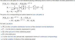
The catch is that the BS formula relies on a few non-realistic assumptions.
Among else, it is assumed that:
a) Interest rates are deterministic
b) The underlying asset price follows a geometric Brownian motion
c) The volatility of the underlying asset price is deterministic
In literature there exist more advanced formulas that relax these assumptions, but they are far too complex to be implemented by a regular user in Excel. Thankfully QuantLib supplies 35 – yes, thirty five (!) – different mathematical models, most of which can calculate option prices in a more advanced fashion than the original BS formula. The problem is the steep learning curve required by the user in order to apply successfully these models on the spreadsheet.
Thankfully again, since August 2017, the Deriscope Excel interface to QuantLib can be employed to price options in Excel using any of the 35 available QuantLib models. The first-time Deriscope user does not need to read any documentation in order to build the related spreadsheets. A few mouse clicks through the Deriscope wizard suffice to create the required formulas!
For example, QuantLib includes the 3-factor Heston Hull White model that treats both interest rates and underlying volatility as stochastic. Using Deriscope, I can easily build a workbook that prices a European Call Option through the Analytic Heston Hull White model as follows:
Step 1:
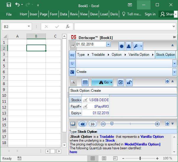
I start by selecting the type "Stock Option" on the Type Selector at the top of the Deriscope wizard as shown below. The Function Selector, located two rows below the Type Selector, is automatically set to the function "Create" and the Browse Area further below displays the mandatory key-value pairs required by that function. These are the Stock, Payoff and Expiry. If I wanted, I could display all key-value pairs – including the optional ones – by clicking on the little button displaying a checked box above the Browse Area.
Step 2:
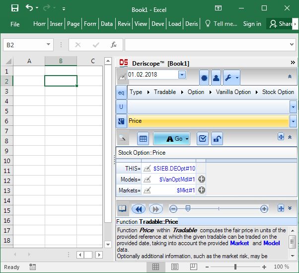
Next I click on the Function Selector and choose the function "Price" from the available list. The result is shown below, where the Function Selector (in orange color) is set to "Price" and the Browse Area displays the mandatory key-value pairs required by the function "Price". These are the THIS, Models and Markets.
Step 3:
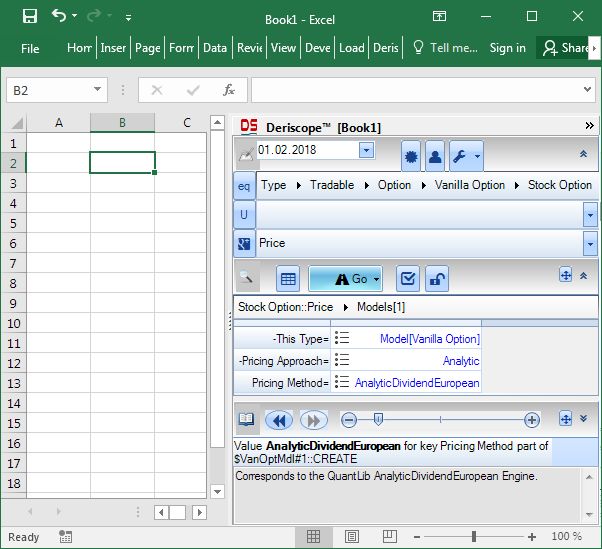
Next I click on the "Pen on a Pad”"sign to the right of the "Models=" key in order to edit the object labelled $VanOptMdl#1 currently presented as a default by Deriscope. Doing so will take me inside the contents of the $VanOptMdl#1 object as shown below:
Step 4:
Since I am interested in the analytic Heston Hull White model, I do not need to change the current value "Analytic" of the "Pricing Approach" key. But I do need to replace the default value "AnalyticDividendEuropean" to the right of the "Pricing Method" key with the new desired method. I simply click on the three horizontal lines and select "AnalyticHestonHullWhite" from the proposed list. The result is as follows:
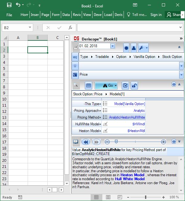
If you are careful enough, you will notice that the wizard has introduced two new key-value pair entries. The new keys are the HullWhite Model and Heston Model. They are needed as they carry the parameters characterizing the Hull & White and Heston models respectively.
You will also notice that the Info Area at the bottom of the Deriscope wizard displays useful information about the selected method, whereby hyperlinks (in blue color) point to more details. This is actually an example of a ubiquitous Deriscope feature, namely the automatic display of local, context-based information as soon as the user makes various selections on the spreadsheet or the wizard.
Step 5:
Finally I click on the "Go" button and then choose "Create Demo Workbook" from the popup menu, as shown here:
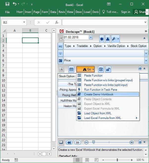
What the "Create Demo Workbook" choice does is to – guess what - create a Demo workbook, which is a brand new Excel workbook being put together on the fly by the Deriscope wizard according to my selections so far. The various spreadsheet formulas are grouped among several sheets according to the type of object they create.
A popular alternative menu choice is the "Paste Function", which pastes all formulas in the same sheet, one below the other, starting with the currently selected cell.
The Demo creation is preferable in complex situations, where several formulas are involved.
The resulting workbook is shown in the next picture. It consists of 5 sheets, where the last one – named "Output" – is selected by default by the wizard as it contains the calculated fair price of the option, 9.934616297, at cell B2.
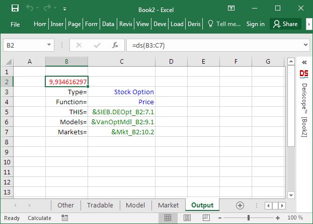
You notice that I have minimized the Deriscope taskpane to the right as I don’t need it any more. Now that all formulas have been created, I can go ahead and edit the various input data as I would do with any other Excel spreadsheet.
The spreadsheet formulas created by the Deriscope wizard are all extremely simple. They all have the syntax "=ds(r1, r2, …)", where r1, r2, … are ranges containing the input data in the form of key-value pairs.
For example, cell B2 in the above picture contains the formula "=ds(B3:C7)", where the range B3:C7 contains 5 key-value pairs that supply the input values for the keys: Type, Function, THIS, Models, Markets. This is all what ds needs to calculate the option price and return the number 9.934616297.
The values corresponding to the keys THIS, Models, Markets contain so called handle names of objects held in Excel memory. They are displayed with green color due to a Deriscope wizard convention to format with green font color all created cells that contain links to other spreadsheet cells. I can change this or any other similar convention in Deriscope Settings if I want.
Let me now select the "Model" sheet and then the cell B2. This is how it looks like:
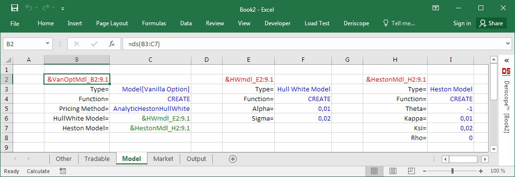
You notice there exist three ds formulas, in cells B2, E2 and H2 respectively.
The formula "=ds(B3:C7)" in cell B2 creates an object of type Model[Vanilla Option], which is the one used in the final formula in the "Output" sheet. As a matter of fact, cell C6 in sheet "Output" simply contains a link to cell B2 here. The object created by the formula in B2 contains the following three pieces of information:
1. Desired pricing method is AnalyticHestonHullWhite
2. Desired Hull & White model is given by the object named &HWmdl_E2:9.1
3. Desired Heston model is given by the object named &HestonMdl_H2:9.1
As you notice, the real parameter specification takes place elsewhere as follows:
The Hull & White model parameters are specified in the object created in cell E2.
The Heston model parameters are specified in the object created in cell H2.
You also notice that Deriscope has used certain default values as input data.
For example, the Alpha parameter of the Hull & White model is set to 0.01 in cell F5 whereas the Theta parameter of the Heston model is set to -1 in cell I5.
You probably have no idea what these parameters exactly mean. You do suspect though that they should somehow influence the pricing result of 9.934616297.
To be honest, even I fail to remember the exact meaning and idiosyncrasies of the various input data. But this is where Deriscope comes to help. All I need to do to know what a certain key-value pair input is for, is open the wizard and select the cell containing the respective key. Doing so for example for the cell H5 containing the key "Theta=", generates the information text at the bottom of the wizard as shown below:

Aha! The mystery about Theta is gone! I know now what this parameter represents.
The information also tells me that a non-positive value acts as a signal to QuantLib to calculate the value of this parameter based on a market implied vol. This means that changing the given value in cell I5 from -1 to -2 should have no effect on the calculated option price. Doing so and then pressing F9 to recalculate the whole spreadsheet actually proves this to be the case.
On the other hand, changing Theta to some positive value should affect the option price. A quick test shows this again to hold.
You may think, this is nice when one only needs to create a workbook dedicated in calculating the price of a single option under a specific model.
Nothing can be further from the truth than that!
It may be true that the Deriscope wizard may only create workbooks dealing with a single derivative instrument and a single pricing model. But after you have access to the building blocks created by the wizard, you can easily put them together and create spreadsheets that deal with several instruments and models. You can afford to do that last step by relying not on Deriscope but on Excel’s ability of pulling things together in a fashion that you alone decide!
As a demonstration of Excel power, I have built a workbook that displays in its last sheet the prices of a one-year European Call Option on a non-dividend-paying stock as calculated by 19 different QuantLib models. You may download this spreadsheet here . The following screenshot shows the table in the last sheet with the comparative option prices.
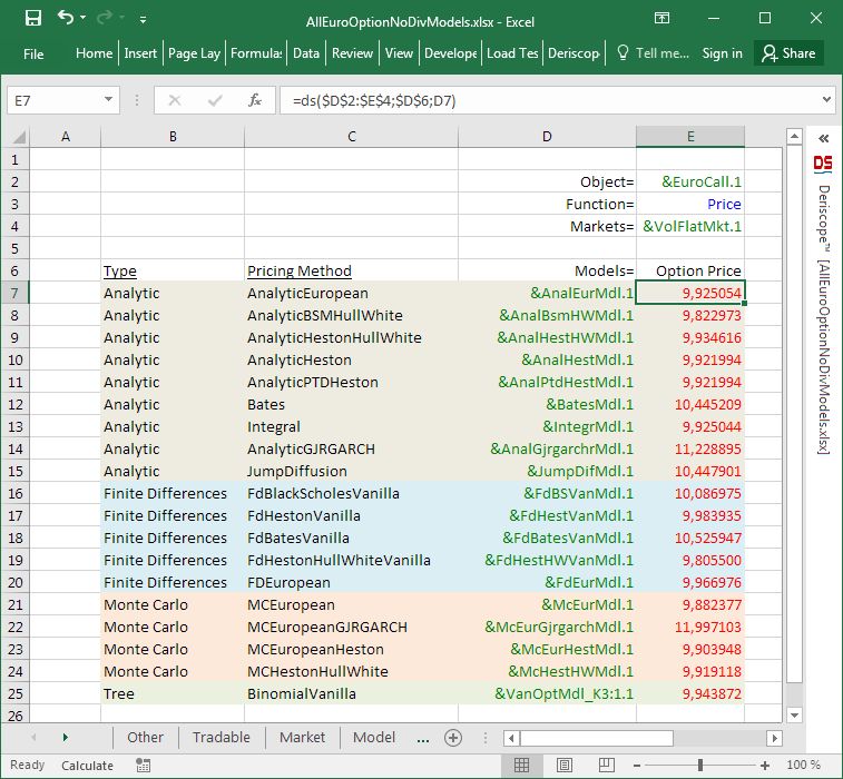
Column E contains the option prices.
Cell E7 is intentionally selected so that you can see the formula “=ds($D$2:$E$4;$D$6;D7)” inside Excel’s formula bar. This is the formula that produces the option price corresponding to the object of type Model[Vanilla Option] in cell D7.
The formula is actually very simple as it takes only three input arguments: the range $D$2:$E$4, the cell $D$6 and the cell D7.
In addition all input ranges except D7 carry the $ sign, which means that only the last input argument D7 changes as this formula is pasted in the cells below E7.
Feel free to contact me if you want to share any thoughts with me with regard to this product or if you want me to add any particular features.
Contact info and social media links are available at my web site https://www.deriscope.com
FinViz - an advanced stock screener (both for technical and fundamental traders)