Numeracy for Traders- Lesson 1 – Fractions

Fractions is a topic from elementary mathematics but surprisingly even some Ph.Ds in math have problems with them. After this lesson you will be able to read pie diagrams, calculate portfolio weights and weighted average returns. This lesson does not substitute systematic learning but helps you to recall fractions and demonstrates their usage in trading context.

To understand fractions is a non-trivial challenge, I myself had problems with them in the secondary school. Moreover, a prominent mathematician Vladimir Arnold has reported that his Ph.D. students in France did have problems with fractions. Most likely this is because fractions are introduced in a secondary school and a teacher usually gives rules how to manipulate them but does not explain the motivation behind. But the mathematical genius Henri Poincaré used to say: it is impossible to master the fractions without (mentally) cutting up an apple or a pie.

Let us first (equally) share a pie among seven friends. Had we seven pies the operation would be elementary: . But we have only one pie, so we need to cut it equally as shown at Figure 1a (by the way, such charts are called pie diagrams). In this sense the fraction is to understand as a directive to divide: i.e. and is essentially the same. In this sense the numerator and the denominator are nothing else but, respectively, the dividend and the divisor.

a	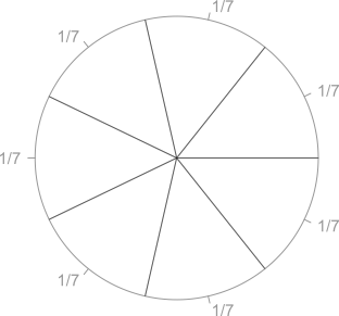b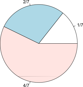
c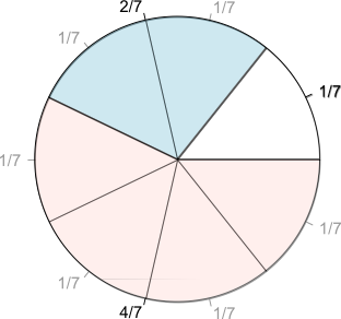
Figure 1: a) equally sharing a pie in 7 parts b) non-equal shares with (common) denominator 7 c) a hint how to add fractions with common denominator

A little bit more complicated case is a non-equal pie sharing. A "pie" may be e.g. the initial capital of a firm: if the first partner invests $10000, the second invests $20000 and the third one invests $40000 then the total capital is and their shares are, respectively, ,  and . Along the way we used an important rule: if the numerator and the denominator have common divisor (in our case it is 10000), we can cancel it. Indeed, the partners' shares remains the same whether they invest $10000, $20000, $40000 or $1, $2, $4. Also from mathematical point of view: a fraction is a directive for division, the result does not change if we multiple both dividend and divisor with a common factor, i.e.our case in .

Now you also (should) easily understand how to multiply fractions: once again, a fraction is a directive to divide, hence
Example 1: if you invest of you capital in a stock index and leave in cash (by zero interest rate, which is not uncommon nowadays) and the index grows by then the total return on your capital is equal to

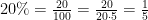
In Example 1 you have also seen how we can convert between common and decimal fractions. In order to convert to a decimal fraction you need to obtain 10, 100, 1000, etc in denominator by multiplying or dividing both denominator and numerator by a common factor. Finding this factor may be a little bit challenging, e.g but don't worry, in practice a calculator or a computer will always do this task for you. As to conversion from a decimal to a common fraction, it is easier: just write in the numerator the digits starting with the first non-zero after the decimal point and in the denominator the factor of 10 with as much zeros as there are digits after the decimal point. E.g. for 0.00105 we write 105 in the numerator (zeros in .00 are omitted, zero in 105 has a non-zero digit left from it, so it is not omitted). There are five digits after the decimal point, so in denominator we write 100000. Finally we may cancel for a common factor 5, so

As to division by a fraction, it is less intuitive (indeed, dividing a pie among "one half" or "two thirds" persons hardly makes sense). But as a mathematical operation it is not uncommon and can be easily formalized: So dividing by is equivalent to multiplying by !

The last rule we need to understand is how to add the fractions with different denominators.

Figure 2: bringing fractions to a common denominator

In order to add and you need first to bring them to the common denominator. You can always do it as follows: .
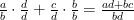
Bringing to a common factor essentially means further (finer) division (or better to say split), as Figure 2 shows. For example, in order to sum and we bring them to the common denominator , which means that one half is split in three parts (so we get three sixths) and two third is split in two, so we get (four sixths) and finally

Sometimes and have a common factor, e.g. you can add and as follows: . But doing is always correct, e.g. in our case .

Finally, let us apply our skill to a task from portfolio management.
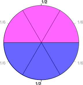
Assume a financial (robo) advisor tells you that you should invest in stocks, in bonds and the rest (which is in gold.
Further assume that the stocks grew by 20%, the bonds gave you 2% of return and the gold grew by 50%. So what is the average return on your investments (or in other words, what is the total return of your portfolio)?!
A naive (innumerate) investor would probably state it is (20% + 2% + 50%) / 3 = 24%. This is, however, wrong. It would be correct if the shares (=weights) of all assets were equal. But generally they are not and we have to calculate the weighted average as follows:

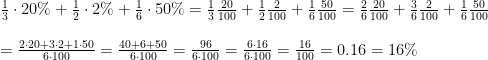
Let's check the correctness of our approach with some concrete numbers. Assume (for computational simplicity) that the initial capital was $60000.
So we put $20000 in stocks, $30000 in bonds and $10000 in gold. These investments, respectively, yielded 20% * $20000 = $4000, 2% * $30000 = $600 and 50% * $10000 = $5000. Total gain in $4000 + $600 + $5000 = $9600. And 9600 / 60000 = 0.16 = 16%, as expected.

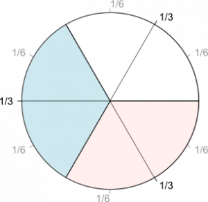
Finally, let us visualize our computations by means of the pie diagrams

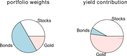
To create Figure 3 I used the following R-code:

#Left-hand pie diagram (initial portfolio weights)
par(mfrow=c(1,2)) #split panel in two (left-right)
slices <- c(1/3, 1/2, 1/6)
lbls <- c("Stocks", "Bonds", "Gold")
pie(slices, labels = lbls, main="portfolio weights")
#right-hand pie diagram (yield contribution)
slices <- c((1/3 * 0.2), (1/2 * 0.02), (1/6 * 0.5))
lbls <- c("Stocks", "Bonds", "Gold")
pie(slices, labels = lbls, main="yield contribution")

Note, however, that the application of the pie diagrams is limited. They are very convenient when you have to visualize the size of shares of a unit, of something holistic. But if some assets had brought a negative return, it would be impossible to use the pie diagram because we cannot visualize negative numbers on them. Moreover, if a unit consists of many parts and some of them have small weights, they may become hardly visible. Thus I, for one, usually prefer the bar plots.