We test different kinds of neural network (vanilla feedforward, convolutional-1D and LSTM) to distinguish samples, which are generated from two different time series models. Contrary to a (naive) expectation, conv1D does much better job than the LSTM.
Currently, the artificial intelligence hype is really enormous and the neural networks experience their (yet another) renaissance. There are also a lot of respective software projects: TensorFlow, Theano, Caffe, MxNet, Deeplearning4j just to name some. A very interesting project is Keras, which allows specifying a neural net model with just a couple of code lines. Keras uses TensorFlow or Theano as a backend, allowing a seamless switching between them. Initially written for Python, Keras is also available in R. Whereas the installation for Python can be tedious, all you have to do in R is to run
devtools::install_github("rstudio/keras")
library(keras)
install_keras()
(Update 2021.02.20: Keras installation in R is not anymore as simple: read this manual
Update 2021.10.17: This simple way to install Keras in R works again!)
Let us generate a marked data sample.
LOOPBACK = 240 #length of series in each sample
N_FILES = 1000 #number of samples
PROB_CLASS_1 = 0.55
SPLT = 0.8 #80% train, 20% test
X = array(0.0, dim=c(N_FILES, LOOPBACK))
Y = array(0, dim=N_FILES) #time series class

for(fl in 1:N_FILES)
{
    z = rbinom(1, 1, PROB_CLASS_1)
    if(z==1)
        X[fl, ] = cumprod(1.0 + rnorm(LOOPBACK, 0.0, 0.01))
    else
        X[fl, ] = exp(rnorm(LOOPBACK, 0.0, 0.05))

    X[fl, ] = X[fl, ] / max(X[fl,]) #rescale
    Y[fl] = z
}
 |
 |
 |
 |
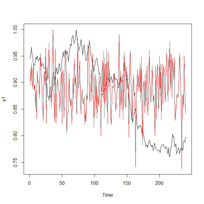
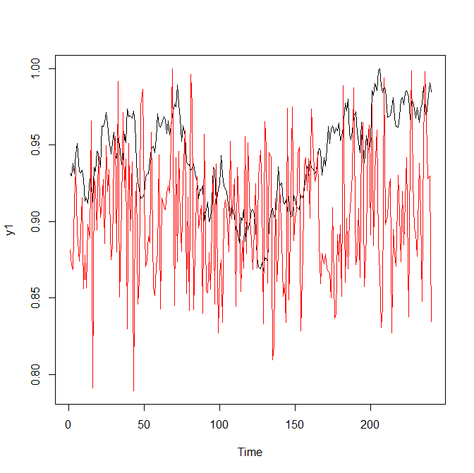
| Figure 1: two classes of time series | |
As you can see, it is not too difficult to discriminate two classes with a naked eye. But let us see how the neural network performs.
We start with a "plain-vanilla" configuration: a feed-forward network with one hidden layer.
library(keras)
b = floor(SPLT*N_FILES)
x_train = X[1:b,]
x_test = X[(b+1):N_FILES,]
y_train = to_categorical(Y[1:b], 2)
y_test = to_categorical(Y[(b+1):N_FILES], 2)

model <- keras_model_sequential()
model %>%
  layer_dense(units = 80, activation = 'relu', input_shape = c(LOOPBACK)) %>%
  layer_dropout(rate = 0.4) %>%
  layer_dense(units = 40, activation = 'relu') %>%
  layer_dropout(rate = 0.3) %>%
  layer_dense(units = 2, activation = 'softmax')
summary(model)
model %>% compile(
  loss = 'categorical_crossentropy',
  optimizer = optimizer_rmsprop(),
  metrics = c('accuracy')
)
history <- model %>% fit(
  x_train, y_train,
  epochs = 60, batch_size = 11,
  validation_split = 0.2
)
plot(history)
model %>% evaluate(x_test, y_test)
It provides an accuracy of 0.595 ... which is not much better than a blind guessing (since we have PROB_CLASS_1 = 0.55). Of course you may (and are encouraged) to experiment with the number of units in the 1st and the 2nd dense layers, dropout rates, optimizer, activation functions and batch_size, but I suspect the result will be the same.
Now let us try a convolutional (conv-1D) neural network.
Convolutional neural networks are mostly (deservedly) fabled in 2D, for their ability to recognize human faces (and from recently also cats and dogs snouts). But in our case the problem is similar: intuitively we feel that the red and black charts in Figure 1 look differently. Fortunately, in order to apply the convolutional neural networks we do not need to "complicate" our problem, making 2D images from 1D time series. Rather we just use a conv1D layer.
In order to do it we have to reshape our data, adding a fictitious 3rd dimension. Why does a conv1D layer require a 3D-tensor as an input? Well, recall the conv2D case: normally the images have three color channels (red, green, blue). Also the time series can have something similar (e.g. Open, High, Low and Close stock prices) thus specifying an additional dimension does make sense.
The number of filters (roughly they can be understood as the distinguishing marks of time series classes) was arbitrary set to 5 (you may experiment with larger and smaller number of filters). The kernel_size was chosen "more deliberately": as you can see at Figure 1, the distances between minima and maxima in the red charts are about 10 steps.
As to layer_max_pooling_1d(pool_size = 4), it just a trade-off between identifying features more sharply and reducing the number of trained weights by 4; layer_flatten() is necessary to flatten a tensor (output of previous layer) into one-dimensional array (Note that you do not need layer_flatten() if you use layer_global_max_pooling_1d()).
Finally we add layer_dense(units = 10, activation = 'relu') to make our network deeper, since currently there is a deep learning hype 🙂
x_train = array_reshape(X[1:b,], c(dim(X[1:b,]), 1))
x_test = array_reshape(X[(b+1):N_FILES,], c(dim(X[(b+1):N_FILES,]), 1))
y_train = to_categorical(Y[1:b], 2)
y_test = to_categorical(Y[(b+1):N_FILES], 2)

model <- keras_model_sequential()
model %>%
  layer_conv_1d(filters=5, kernel_size=10,  activation = "relu",  input_shape=c(LOOPBACK, 1)) %>%
  #layer_global_max_pooling_1d() %>%
  layer_max_pooling_1d(pool_size = 4) %>%
  layer_flatten() %>%
  layer_dense(units = 10, activation = 'relu') %>%
  layer_dense(units = 2, activation = 'softmax')
summary(model)
model %>% compile(
  loss = 'categorical_crossentropy',
  optimizer = optimizer_rmsprop(),
  metrics = c('accuracy')
)
history <- model %>% fit(
  x_train, y_train,
  epochs = 60, batch_size = 30,
  validation_split = 0.2
)
plot(history)
model %>% evaluate(x_test, y_test)
And how about the results?! Well, they are impressive, after 12 epochs the accuracy converges to 1, which means that our neural network has really good eyes :).
Finally, let us try the LSTM model.
model <- keras_model_sequential()
model %>%
  layer_lstm(units = 24, input_shape=c(LOOPBACK, 1)) %>%
  layer_dense(units = 2, activation = 'sigmoid')

summary(model)
model %>% compile(
  loss = 'categorical_crossentropy',
  optimizer = optimizer_rmsprop(),
  metrics = c('accuracy')
)
history <- model %>% fit(
  x_train, y_train,
  epochs = 60, batch_size = 24,
  validation_split = 0.2
)
plot(history)
model %>% evaluate(x_test, y_test)
"Surprisingly" it gives even worse accuracy than the plain-vanilla feedforward network. I say "surprisingly" because LSTM (as a kind of RNN) are fabled for capturing the serial dependence in timeseries. This is though correct, but look: both classes of our time series are actually the processes with independent increments! Thus one shall hardly expect that an RNN will perform well in our case.
P.S.
You might say, a nice case study but is it really practical? Finally, we want first of all to predict a time series. Yes, it is practical. I, for one, had to classify the load curves of gas consumers as I worked for an energy company. And in trading (where the price prediction is rarely possible, if at all) the classification task may also be relevant. Stay tuned!
FinViz - an advanced stock screener (both for technical and fundamental traders)