In our previous post on Nelson-Siegel model we have shown some pitfalls of it. In this follow-up we will discuss how to circumvent them and how machine learning and artificial intelligence can[not] help.
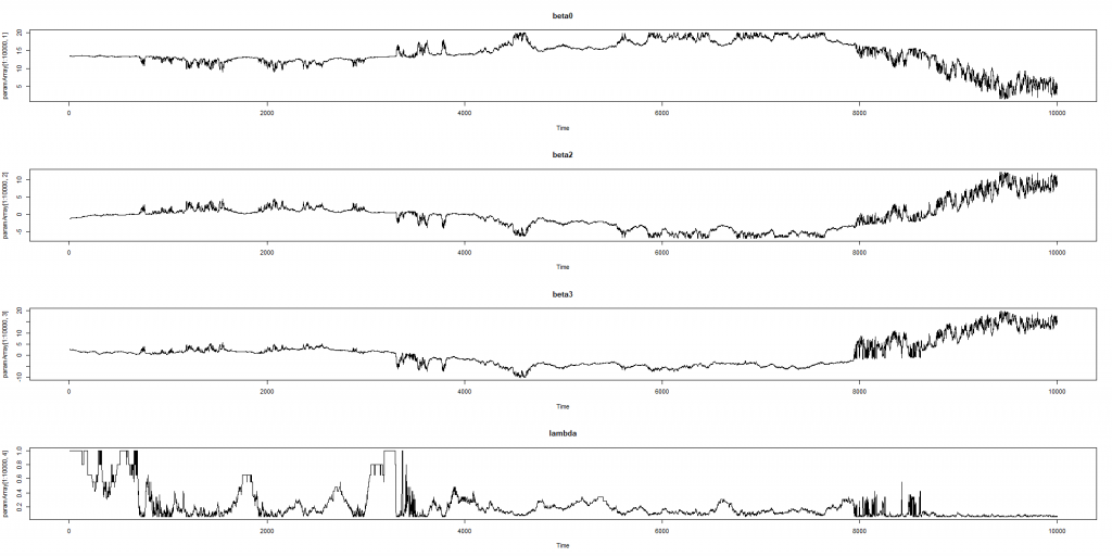
In the previous part we have provided an example of convergence failure of R-library YieldCurve. You may wonder how we come came across this example. Well, Monte-Carlo simulation helped us:
library(YieldCurve)

#Start with sample values for FedYieldCurve on 1982-04-30
data(FedYieldCurve)
rate.Fed = first(FedYieldCurve,'5 month')
maturity.Fed <- c(3/12, 0.5, 1,2,3,5,7,10)
NSParameters <- Nelson.Siegel( rate= rate.Fed, maturity=maturity.Fed )
pp = NSParameters[5,] #parameters ins xts format

MATURITY_BASES = c(0.25, 0.5, 1, 1.5, 2, 3, 4, 5, 7, 10, 12, 15, 20, 25, 30) #maturities in years
VOLAs = 0.005*sqrt(MATURITY_BASES) #volatilies (they grow at sqrt-speed as time grows)
VOLAs[1:3] = VOLAs[1:3]*c(4,3,2) #short end is usually more volatile
N_MAT = length(MATURITY_BASES) #number of matutiries

N_SIMULATIONS = 1e5
paramArray = array(0.0, dim=c(N_SIMULATIONS, 4)) #log NS params for each simulation
oldYieldsArray = array(0.0, dim=c(N_SIMULATIONS, N_MAT))
newYieldsArray = array(0.0, dim=c(N_SIMULATIONS, N_MAT))
newNsYieldsArray = array(0.0, dim=c(N_SIMULATIONS, N_MAT))
maxDistanceArray = array(0.0, dim=N_SIMULATIONS)
relativeMaxDistanceArray = array(0.0, dim=N_SIMULATIONS)

for(j in 1:N_SIMULATIONS)
{
    oldYields = NSrates(pp, MATURITY_BASES)
    newYields = oldYields + rnorm(N_MAT, rep(0.0, N_MAT), VOLAs)
    newMATs = MATURITY_BASES - 1.0/365 #next day all mats become 1 day shorter
    pp = Nelson.Siegel(newYields, newMATs)
    newNsYields = NSrates(pp, newMATs)

    npo = c(newYields, oldYields)
    plot(MATURITY_BASES, oldYields, ylim=c(min(npo), max(npo)))
    lines(MATURITY_BASES, oldYields)
    points(MATURITY_BASES, newYields, col="red", pch=4)
    points(newMATs, newNsYields, col="blue")
    lines(newMATs, newNsYields, col="blue")

    oldYieldsArray[j,] = as.numeric(oldYields)
    newYieldsArray[j,] = as.numeric(newYields)
    newNsYieldsArray[j,] = as.numeric(newNsYields)
    maxDistanceArray[j] = max( abs(oldYieldsArray[j,] - newNsYieldsArray[j,]) )
    relativeMaxDistanceArray[j] =  maxDistanceArray[j] / max(abs(oldYieldsArray[j,]))
    paramArray[j,] = as.numeric(pp)
}

plot(density(maxDistanceArray))
plot(density(log(maxDistanceArray)))
idx=which.max(maxDistanceArray)
maxDistanceArray[which.max(maxDistanceArray)]
relativeMaxDistanceArray[which.max(relativeMaxDistanceArray)]
What we essentially do is the following: we start with some yield curve (the choice of Fed curve on 1982-04-30 is pretty arbitrary), then step-by-step randomly modify the yields and finally try to fit the NS model to the new yields. It is not uncommon to compare the curve on current and previous days, so we essentially simulate this.
oldYields = NSrates(pp, MATURITY_BASES)

newYields = oldYields + rnorm(N_MAT, rep(0.0, N_MAT), VOLAs)

newMATs = MATURITY_BASES - 1.0/365 #next day all mats become 1 day shorter

pp = Nelson.Siegel(newYields, newMATs)

newNsYields = NSrates(pp, newMATs)
This simulation also allowed us to record this video, which demonstrates that the universe of NS-Curves is pretty rich.
Note that this Monte-Carlo simulation is in a sense "benevolent" for the Nelson-Siegel model because we always assume that the yields on previous step (oldYields) are perfectly matched by an NS-curve. But even this benevolence does not help to avoid troubles completely. How do we detect these troubles? Easily! On each step we calculate the maximal distance (supremum-norm) between two adjacent curves:
maxDistanceArray[j] = max( abs(oldYieldsArray[j,] - newNsYieldsArray[j,]) )
In the end we just find the step on which the maximum distance to the previous curve and this is the example of convergence failure, given in the previous post.
Ok, problem detected, but what to do to solve it? A not implausible idea may be to engage the machine learning and teach e.g. a neural network to detect such cases. Moreover, it seems very promising that we can allegedly avoid a tiresome work to mark our training set. However, the probability density of the maxDistanceArray looks as follows:

Distribution tail is visually diminishing at 0.08 but a daily shift by 8 basis points is not uncommon for a yield curve. Thus, although we did 1e5=10000 Monte-Carlo simulations, we got just few extreme cases, which we can mark as bad. And it is definitely insufficient to train a neural network. Moreover, as we previously noted, two Nelson-Siegel curves may lie pretty close to each other but have their parameters far away from each other. So can this probably be a starting point?

Since the model is linear in it is plausible to assume that extremely high changes in betas (e.g. beyond 95-quantile) are outliers and mark them as bad.
mmScaler <- function(x){(x-min(x))/(max(x)-min(x))}  #MinMaxScaler
beta0_ds= abs(diff(paramArray[1:N_SIMULATIONS,1])) / abs(paramArray[1:(N_SIMULATIONS-1),1])
beta1_ds= abs(diff(paramArray[1:N_SIMULATIONS,2])) / abs(paramArray[1:(N_SIMULATIONS-1),1])
beta2_ds= abs(diff(paramArray[1:N_SIMULATIONS,3])) / abs(paramArray[1:(N_SIMULATIONS-1),1])

b0 = mmScaler(beta0_ds)
b1 = mmScaler(beta1_ds)
b2 = mmScaler(beta2_ds)

#now filter out jumping betas
QUANTILE = 0.95
q_b0 = as.numeric(quantile(b0, QUANTILE))
q_b1 = as.numeric(quantile(b1, QUANTILE))
q_b2 = as.numeric(quantile(b2, QUANTILE))
idx = intersect(intersect(which(b0 < q_b0), which(b1 < q_b1)), which(b2 < q_b2))
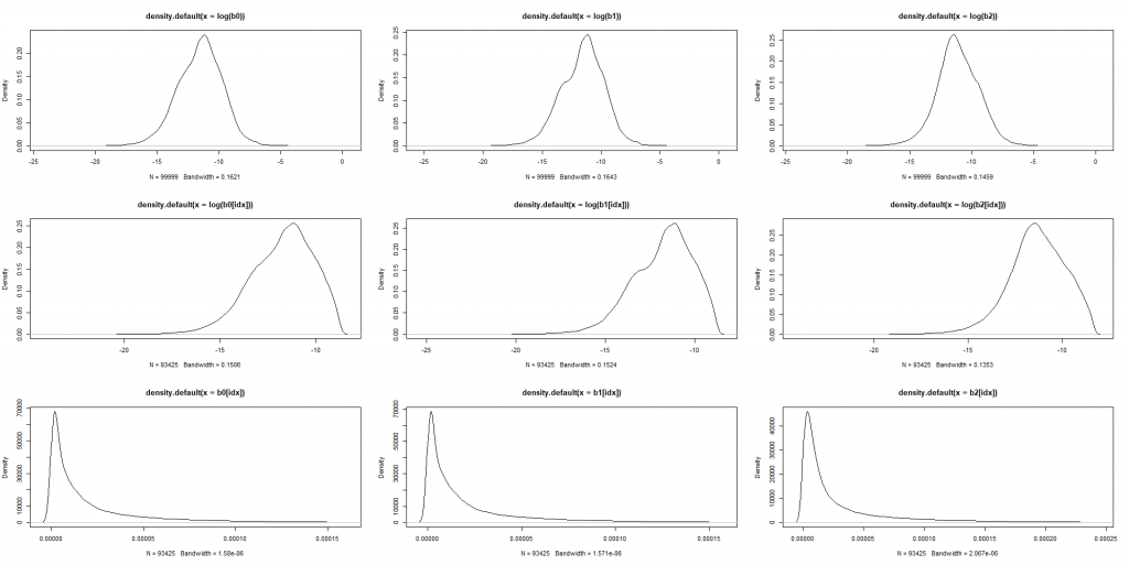
par(mfrow=c(3,3))
plot(density(log(b0)))
plot(density(log(b1)))
plot(density(log(b2)))
plot(density(log(b0[idx])))
plot(density(log(b1[idx])))
plot(density(log(b2[idx])))
plot(density(b0[idx]))
plot(density(b1[idx]))
plot(density(b2[idx]))

#de-mean
b0 = b0-mean(b0)
b1 = b1-mean(b1)
b2 = b2-mean(b2)

#train neural network
X = cbind(b0, b1, b2)
Y = array(0, dim=(N_SIMULATIONS-1))
Y[idx] = 1

Then we can train a neural network
SPLT = 0.8
library(keras)
b = floor(SPLT*(N_SIMULATIONS-1))

x_train = X[1:b, ]
x_test = X[(b+1):(N_SIMULATIONS-1), ]
y_train = to_categorical(Y[1:b], 2)
y_test = to_categorical(Y[(b+1):(N_SIMULATIONS-1)], 2)

model <- keras_model_sequential()
model %>%
  layer_dense(units = 3, activation = 'tanh', input_shape = dim(X)[2]) %>%
  layer_dense(units = 2, activation = 'tanh') %>%  #relu here (sometimes) gives slightly better accuracy than tanh
  layer_dense(units = 2, activation = 'softmax')
summary(model)
model %>% compile(
  loss = 'categorical_crossentropy',
  optimizer = optimizer_rmsprop(),
  metrics = c('accuracy')
)
history <- model %>% fit(
  x_train, y_train,
  epochs = 100, batch_size = 100,
  validation_split = 0.2
)
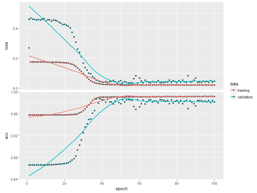
plot(history)
model %>% evaluate(x_test, y_test)

The neural network provides a high accuracy not only in-sample but also on validation set (0.9825) ... but only for THIS data set.
If you simulate a new dataset, e.g. modifying VOLAs = 0.005*sqrt(MATURITY_BASES) to VOLAs = 0.05*sqrt(MATURITY_BASES) the model will fail to recognize the bad cases on the new dataset. You can (and are encouraged to) check this as follows:
#####################################
###load new workspace at this step###
#####################################
beta0_ds_2 = abs(diff(paramArray[1:N_SIMULATIONS,1])) / abs(paramArray[1:(N_SIMULATIONS-1),1])
beta1_ds_2 = abs(diff(paramArray[1:N_SIMULATIONS,2])) / abs(paramArray[1:(N_SIMULATIONS-1),2])
beta2_ds_2 = abs(diff(paramArray[1:N_SIMULATIONS,3])) / abs(paramArray[1:(N_SIMULATIONS-1),3])
b0_2 = mmScaler(beta0_ds_2)
b0_2 = b0_2 - mean(b0_2)
b1_2 = mmScaler(beta1_ds_2)
b1_2 = b1_2 - mean(b1_2)
b2_2 = mmScaler(beta2_ds_2)
b2_2 = b2_2 - mean(b2_2)

X2 = cbind(b0_2, b1_2, b2_2)
result = model %>% predict(X2)
idxRes = which(round(result[,1]) == 1)
The problem is: although we normalize and demean the data in both cases, a linear change in model volatility has a highly non-linear effect on tail-quantiles. That's why data normalization hardly helps.
So do we need a more complex AI-model (which tries to learn the volatility impact on higher quarantines)? Well, it might work (but imagine how many Monte Carlo simulation you need to train this model). Maybe, a simpler approach is better: e.g. just keep your eye on and if it jumps, try to fix it to the median of previous 10 days and then fit betas. Worked for Nelson and Siegel, thus will likely work for you 🙂
FinViz - an advanced stock screener (both for technical and fundamental traders)
