The Highest Volatility in October? Don’t trust a Superficial Statistics!

A recent post "Fasten your seat belt for stocks: October is almost here" on MarketWatch, repeated by Morningstar and shared in my social networks may make an illusion that it is likely to expect high(est) volatility in October. A little bit more detailed statistical analysis shows that such expectation is superficial.
A more general (and very old) lesson from this case: the statistical analysis is much more than a primitive consideration of the mean values in groups. And of course: don't trust provoking titles.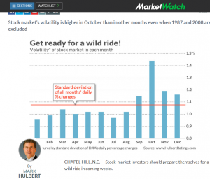

A recent post by Mark Hulbert on MarketWatch, also repeated by MorningStar may give an impression that it is plausible to expect a high volatility also in coming October (2018). Whereas it indeed might be the case (e.g. due to the trade war between China and USA), there is no significant pattern in time series of market returns.

First of all in order get a better insight it is useful to plot not just average volatility values of daily returns aggregated per month but a boxplot of daily returns aggregated per month.

library(alphavantager)
av_api_key("your_key_here")
spy=av_get(symbol = "SPY", av_fun = "TIME_SERIES_DAILY_ADJUSTED", outputsize = "full")
xxx = xts(spy$adjusted_close, order.by=spy$timestamp)
chartSeries(xxx)
##
rrr = dailyReturn(xxx)
months = substr(index(rrr),6,7)
LST = list()
LST2 = xts()
for(mm in 1:12)
{
    rrmm = rrr[which(as.numeric(months)==mm)]
    LST[[mm]] = rrmm
    N = length(rrmm)
    idx = (sort(as.numeric(rrmm), index.return=TRUE))$ix
    rrmm2 = (rrmm[idx[2:(N-2)]])
    LST2 = append(LST2, rrmm2)
    print(sd(rrmm2) )
}
boxplot(as.numeric(LST2) ~ substr(index(LST2),6,7))
abline(v=10, col="red")

Then you readily see that although the volatility in October is indeed somethat higher, it is mostly due to the outliers, which come rarely and unpredictably. Reminder: the estimation of the volatility (which is, in essence, just the standard deviation of returns) is very sensitive to outliers.

Even better insight gives you the time series of monthly boxplot, you merely need a big screen to grasp this pdf.
In particular, note that the last two Octobers were actually very calm.

library(alphavantager)
av_api_key("your_key_here")
spy=av_get(symbol = "SPY", av_fun = "TIME_SERIES_DAILY_ADJUSTED", outputsize = "full")
library(quantmod)
xxx = xts(spy$adjusted_close, order.by=spy$timestamp)
chartSeries(xxx)
##
rrr = dailyReturn(xxx)
mmyyyy = substr(index(xxx),1,7)
##
pdf(file="C:/R/octoberVola.pdf", width=40, height=32)
boxplot(as.numeric(rrr) ~ mmyyyy, las=2)
abline(v=seq(from=10, to=290, by=12), col="red") #mark Octobers (alphavantage provides data on SPY from Jan 95)
dev.off()

P.S.
If you are looking for a deeper analysis of market volatility, have a look at this!