Reproducing a Pseudo-Random Walk down the Wall Street

Malkiel affirms that the stock returns follow the random walk. Lo and MacKinlay retort they do not.
In this post I show how a mean-reverting process can be efficiently disguised as a random walk. Most likely, the market does follow a similar disguise-pattern (at least sometimes).

Being a strong supporter for Lo's and MacKinlay's view I nevertheless emphasize that both studies lack reproducibility and impartiality. The former problem is not necessary due to the unwillingness of the authors to make their research reproducible but first of all due to a restrictive licensing of the market data. As to the latter, Burton G. Malkiel spent 28 years as a director of the Vanguard Group, which pioneered index funds (and thus propagandized passive investment in ETFs). As to Andrew Lo, his cui bono cannot be as straightforwardly deduced from his affiliations but he definitely made a strong goodwill by being a prominent disputant of the efficient market hypothesis.

Anyway, inspired by the experimental archaeology, let us state the question as follows: can the stock returns, being (sometimes) exploitable, disguise themselves as a random walk?!.
Well, probably yes! Let us generate a path of stochastic process as follows:
1. Generate the 1st segment of a random walk with a random length upto MAX_PIECE_LEN (this segment mimics the stock returns, to mimic the prices in a simplistic way we take the cumsum of returns).
2. LOOP
Generate the next segment of a random walk with a random length upto MAX_PIECE_LEN, cumsum and append it to the path IF it eventually goes down AND the previuos segment went up or vice versa (otherwise just skip this segment and CONTINUE)

pseudoRandomWalk <- function(N_PIECES = 50, MAX_PIECE_LEN = 30)
{
    piece = rnorm(sample(2:MAX_PIECE_LEN, 1), 0, 1)
    res = cumsum(piece)
    totalRes = list()
    totalRes = append(totalRes, res)
    turnArounds = list()
    turnArounds = append(turnArounds, length(piece))
    p=1
    while(p<N_PIECES)
    {
        newPiece = rnorm(sample(2:MAX_PIECE_LEN, 1), 0, 1)
        newRes = cumsum(newPiece) + tail(res, 1)
        if(res[1] > tail(res, 1))
        {
            if(newRes[1] > tail(newRes, 1)) {
                next
            } else {
                res = newRes
                turnArounds = append(turnArounds, length(newPiece))
                totalRes = append(totalRes, res)
                p = p+1
            }

        } else if(res[1] < tail(res, 1))
        {
            if(newRes[1] < tail(newRes, 1)) {
                next
            } else {
                res = newRes
                turnArounds = append(turnArounds, length(newPiece))
                totalRes = append(totalRes, res)
                p = p+1
            }
        }
    }

    return(list(totalRes, turnArounds))
}

The following sketch, which is obtained by

res = pseudoRandomWalk(7)
stockPrice = unlist(res[[1]])
vantagePoints = cumsum(unlist(res[[2]]))
ts.plot(stockPrice, main="A pseudo random walk")
abline(v=vantagePoints, lty="dotted")

shall demonstrate the idea visually

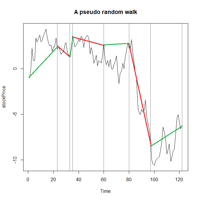
Note that only the terminal states of segments matter: e.g. the last segment (which finally goes up) first continues to fall.

Now let us generate a longer but still a not-so-long path. This is exactly what we have to deal with on the market: the long series of financial data may not be available at all and even if, the relevance of the not-so-recent history is questionable.

res = pseudoRandomWalk(500)
stockPrice = unlist(res[[1]])
par(mfrow=c(1,2))
S = length(stockPrice)
acf(diff(stockPrice), main=paste("ACF of the Pseudo-RW:", S, "samples"))
acf(rnorm(S, mean(stockPrice), sd(stockPrice)), main="ACF of a genuine RW")

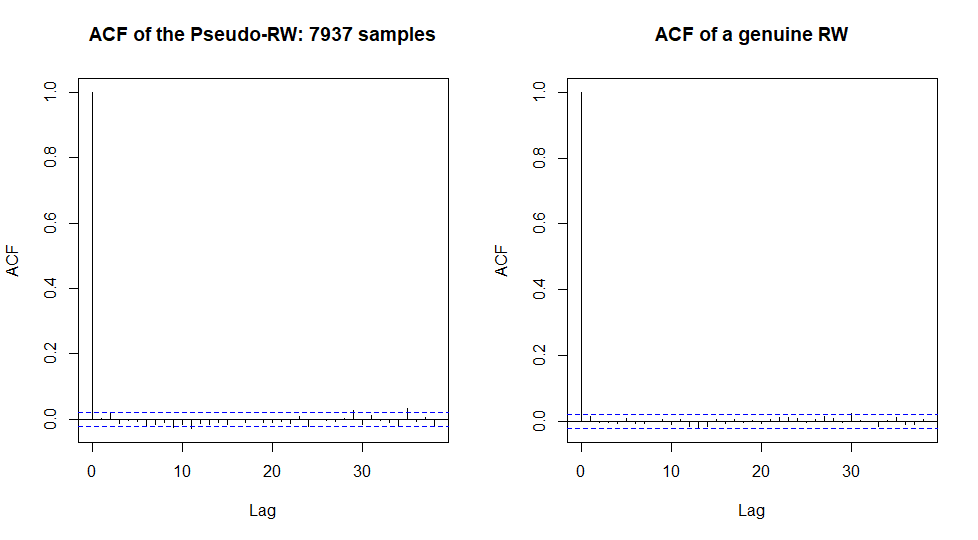
Do you see the difference? Well, to be true I ran the R code several times to get especially nice case. And yes, the series of the negative autocorrelations around 10 on the left-hand chart may catch an eye. But anyway these autocorrelations are still within the confidence band, which means that they may be purely random. Note that we have 7937 samples in our "history", which is a pretty big number. Of course, if we increase it more and more then the law of large numbers will eventually do its job and reveal the genuine autocovariance function of our process.

But once again: in practice with usually have to deal with pretty limited samples.

Further let us try to recognize the "imposter" with "more formal" statistical tests, which are less ambiguous than the visual analysis (there is still some ambiguity due to the choice of the confidence levels).

So running

res = pseudoRandomWalk(500)
stockPrice = unlist(res[[1]])
S = length(stockPrice)
print(paste0("sample length: ",S))
library(tseries)
adf.test(diff(stockPrice))
kpss.test(diff(stockPrice))
library(longmemo) #test Hurst Exponent
d  <- WhittleEst(diff(stockPrice))
confint(d)

gives us

> res = pseudoRandomWalk(500)
> stockPrice = unlist(res[[1]])
> S = length(stockPrice)
> print(paste0("sample length: ",S))
[1] "sample length: 7821"
> library(tseries)
> adf.test(diff(stockPrice))

Warning message:
In kpss.test(diff(stockPrice)) : p-value greater than printed p-value
> library(longmemo) #test Hurst Exponent
> d <- WhittleEst(diff(stockPrice)) > confint(d)
2.5 % 97.5 %
H 0.4753415 0.5028877

It seems that (only) the Augmented Dickey-Fuller Test does a good job but I suspect there is merely a buggy implementation of it (or likely I misinterpret the small p-value). Anyway, as I ran adf.test(rnorm(7821)) I also got p-value = 0.01

> adf.test(rnorm(7821))

Warning message:
In adf.test(rnorm(7821)) : p-value smaller than printed p-value


Finally let us test the Lo-Mac test from their seminal paper.
This test indeed does a good job!

library(vrtest)
Boot.test(diff(stockPrice), kvec=c(2:30), nboot=100, wild="Normal", prob=c(0.025,0.975))
#vs p-values of
Boot.test(rnorm(S), kvec=c(2:30), nboot=100, wild="Normal", prob=c(0.025,0.975))

However, if I reduce the sample length to ca. 1500 elements, I can cheet the LoMac test, too.

> res = pseudoRandomWalk(100)
> stockPrice = unlist(res[[1]])
> S = length(stockPrice)
> S
[1] 1491
> Boot.test(diff(stockPrice), kvec=c(2:30), nboot=100, wild="Normal", prob=c(0.025,0.975))
$`Holding.Period`
[1] 2 3 4 5 6 7 8 9 10 11 12 13 14 15 16 17 18 19 20 21 22 23 24 25 26 27 28 29 30

$CD.pval
[1] 0.08

You may say: ok, but even if the underlying stochastic process is not a random walk, it does not yet automatically imply that it can be exploited. Yes, that is correct but let us try to find an exploiting strategy. Note that all we assume is that we know that the process is somehow mean-reverting in a not-so-long term and we do NOT know the array of vantage points.
We engage the Bollinger bands, selling when the "price" hits the upper band and buying when it touches the lower band.

library(TTR)
N_SIMULATIONS = 1000
TRADING_RES = array(0.0, dim=N_SIMULATIONS)
for(ss in 1:N_SIMULATIONS)
{
stockPrice = unlist(pseudoRandomWalk(100)[[1]])
bought = FALSE
sold = FALSE
buyPrice = list()
sellPrice = list()

for(k in 201:600)
{
  bollinger = BBands(stockPrice[(k-200):k])
  if((stockPrice[k] > tail(bollinger[, 3], 1)) && !sold) #>up, sell
  {
      sold = TRUE
      bought = FALSE
      sellPrice = append(sellPrice, stockPrice[k])
  }
  if((stockPrice[k] < tail(bollinger[, 1], 1)) && !bought) #<down, buy
  {
      sold = FALSE
      bought = TRUE
      buyPrice = append(buyPrice, stockPrice[k])
  }

  if(k==600 && (length(unlist(buyPrice)) != length(unlist(sellPrice))))
  {
      if(sold) {
         buyPrice = append(buyPrice, stockPrice[k])
      }
      if(bought)
      {
          sellPrice = append(sellPrice, stockPrice[k])
      }
  }
}
unlist(buyPrice)
unlist(sellPrice)
TRADING_RES[ss] = sum(unlist(sellPrice) - unlist(buyPrice))
}   
plot(density(TRADING_RES), "PnL distribution with mean and +/- 3 sigmas")
mu = mean(TRADING_RES)
sigma3 = 3*sd(TRADING_RES)
abline(v = c(mu, mu-sigma3, mu+sigma3))

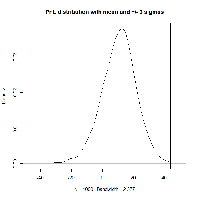
Note that we can (to some extend) exploit the mean-reversion on relatively short samples, on which even the LoMac test fails! "Exploit" does not mean to make profit for sure but even such a simple trading strategy does generate a positive mean.

Dear Pythonistas (esp. those, who used to offend the R-language),
A modern working quant and data scientist shall likely possess both R and Python. So I did my best to re-write my generator of the pseudoRandomWalk in Python, I even tried to make my code neater (what I did not for my R code draft).

from typing import List
from typing import Tuple
import numpy as np
import matplotlib.pyplot as plt

def pseudoRandomWalk(nPieces: int, maxPieceLen: int) -> Tuple[float, int]:
    piece: List[float] = np.random.normal(0, 1, np.random.randint(2, maxPieceLen+1))
    res: List[float] = np.cumsum(piece).tolist()
    totalRes: List[float] = [res] #[] because of further flatting
    turnArounds: List[int] = [len(piece)]
    
    newRes: List[float] = []
    p: int = 2
    while(p < nPieces):
        piece = np.random.normal(0, 1, np.random.randint(2, maxPieceLen+1))
        newRes = [x+res[-1] for x in np.cumsum(piece)] #add tail(res, 1) to cumsum(piece)
        
        if(res[0] >= res[-1]):
            if(newRes[0] > newRes[-1]):
                continue
        elif (res[0] < res[-1]):
            if(newRes[0] < res[-1]):
                continue
            
        res = newRes
        turnArounds.append(len(piece)) #appending a scalar is not a problem
        totalRes.append(res)
        p += 1                   
        
    return totalRes, turnArounds
    
(pathPieces, turnArounds) = pseudoRandomWalk(7, 30)
process = sum(pathPieces, []) #list of list, generated by append must be flattened
vantagePoints = np.cumsum(turnArounds)
plt.plot(np.arange(1, len(process)+1), np.array(process))
for vl in vantagePoints:
    plt.axvline(x=vl, linestyle='--')
plt.show()