In many countries a mortgage shall be completely redeemed to the end of its duration and may be refinanced anytime. In USA one additionally can foreclose his mortgage by mailing his house-keys to a bank. In Germany is different.
First of all, one may completely refinance a mortgage only after 10 years (otherwise one have to pay Vorfälligkeitsentschädigung - a compensation to a bank for missed interest). But taking a long-term mortgage (20 or 30 years) implies a higher mortgage rate, thus it is not uncommon to take several consequent 10- (or sometimes even 5-) year mortgages. In order to optimize mortgage costs / rate change risk relation one can take several submortgages with different durations. Last but not least there is no requirement to amortize a mortgage completely: normally one refinances the residual debt (Restschuld) with a follow-up mortgage (Anschlussfinanzierung).
In this post we discuss the challenges of mortgage optimization and show how two popular programming languages - R and Python - can help us together
Even though the banks do not allow a completely flexible choice of submortgages but rather usually offer 2 or 3 alternatives, it is not easy to make the optimal choice. Let us start with a concrete example: assuming €300000 loan and monthly installment of €1000 what is better - a (sub)mortgage for 20 years by 1.28% p.a. or for 30 years by 1.58%?! Since the rate difference is "merely" 0.3%, a typical risk averse (as well as financially illiteral and innumerate) German usually prefers the latter. Indeed, the second alternative provides a fixed rate (Zinssicherheit) for 30 years, whereas the first one "only" for 20 years. But let us calculate a break-even forward(20, 10) rate, i.e. let us assume that we take a 20Y mortgage and in 20 years refinance it with a follow-up 10Y mortgage by (so far unknown) rate. It turns out that as far as this rate remains under 3.86%, the 20Y mortgage is preferable!
but remember: a human being has no (indigenous) intuition for the exponential function! If at all, there is such intuition only for the speed 


Note however that the forward breakeven mortgage rate also does depend on the credit volume and monthly installment (and not only on yield-to-maturity difference). Indeed, assuming (as before) €300000 loan but reducing the monthly installment to €800 results in the breakeven forward mortgage rate of 2.86%... which is not too improbable in 20 years!
In order to help people make suchlike estimations, we have developed a tool (available both in German and English). However, it does not allow a simultaneous calculation of several submortgages. Neither it provides a stochastic mortgage rate simulation nor a nice visualization of results. Thus we developed a next-generation tool, which does have it all.
But let us first reproduce the above-mentioned example.
import numpy as np
from scipy.optimize import fsolve #https://stackoverflow.com/questions/10652675/solving-an-equation-with-scipys-fsolve

class Zinser:
   longDebt = 0.0       #residual debt by the long-term mortgage rate binding
   shortDebt = 0.0      #residual debt by the short-term mortgage rate binding
   notional = 0.0       #mortgage sum
   installment = 0.0    #monthly installment
   shortRate = 0.0      #mortgage rate p.a. by the short-term mortgage rate binding
   longRate = 0.0       #mortgage rate p.a. by the long-term mortgage rate binding
   shortDuration = 0    #short mortgage duration in years
   longDuration = 0     #long mortgage duration in years
   forwardDebt = 0      #auxiliary variable to iterate, must converge to longDebt
   forwardRate = 0      #breakeven forward mortgage rate, i.e. longDebt = shortDebt + restshuldVonAnschlussFinanzierung.
                        # !NB it depends on all mortgage parameters (on notional and installment as well, and not only on shortRate, longRate and durationDiff as by 'canonical' forward rates)


   def __init__(self, notional, installment, shortRate, shortDuration, longRate, longDuration):
        self.longDebt = notional
        self.shortDebt = notional
        self.notional = notional
        self.installment = installment
        self.shortRate = shortRate
        self.longRate = longRate
        self.shortDuration = shortDuration
        self.longDuration = longDuration

        for ml in range(12*longDuration):
            self.longDebt -= (installment - self.longDebt * longRate/12) #ToDo: break if the debt becomes negative

        for ms in range(12*shortDuration):
            self.shortDebt -= (installment - self.shortDebt * shortRate/12)

        self.forwardRate = fsolve(self.iterateForwardZins, shortRate)


   def iterateForwardZins(self, forwardRate):
        self.forwardDebt = self.shortDebt
        durationDiff = self.longDuration - self.shortDuration
        for ma in range(12*durationDiff):
            self.forwardDebt -= (self.installment  -  self.forwardDebt*forwardRate/12)

        #print(self.forwardRate) #for debugging
        return self.longDebt - self.forwardDebt

v1 = Zinser(3e5, 800, 0.0128, 20, 0.0158, 30)
v1.forwardRate
Out[15]: array([0.02860649])

v2 = Zinser(3e5, 1000, 0.0128, 20, 0.0158, 30)
v2.forwardRate
Out[21]: array([0.03857974])
In my opinion the advantages of the object-oriented programming in this case are obvious: in order to find the optimal solution we need to deal with many submorgages, which are somewhat complex structures so that is better to keeps them as objects (rather than e.g. as a list of lists). In the sense of OOP Python has a clear advantage over R. But do you know a (proven) Python implementation of a Cox-Ingersoll-Ross (CIR) stochastic process? And such a powerful visualization tool as Shiny (and even if, how about a service like shinyapps.io)?!
Thus our further goal is to integrate R and Python. Fortunately, there is an excellent R-package for this: https://rstudio.github.io/reticulate/
I recommend to install it from GitHub: remotes::install_github("rstudio/reticulate", force = T, ref = '0a516f571721c1219929b3d3f58139fb9206a3bd')
otherwise it chooses a wrong version of Python and you will get something like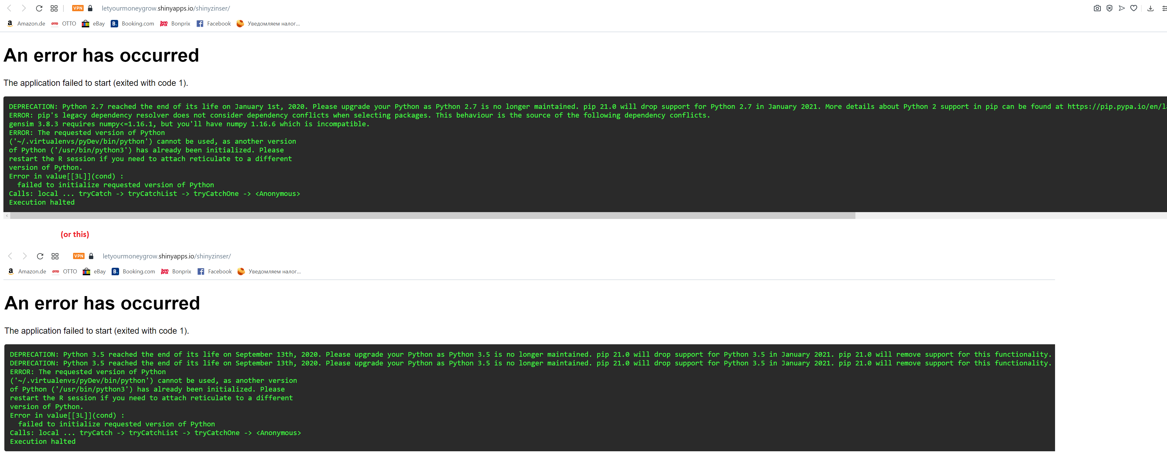
See also https://stackoverflow.com/questions/54651700/use-python-3-in-reticulate-on-shinyapps-io
Further we need to configure the virtual Python environment in our shiny app. By some trial and error I came to the following solution for shinyapp.io
library(reticulate)
virtualenv_create('pyDev')
virtualenv_install("pyDev", packages = c('numpy','scipy'))
use_virtualenv("pyDev", required = TRUE)
import('numpy')
source_python('bauFinanzierungForwardZinsRechner.py')
On a local machine one can explicitly specify, which Python interpreter to use:
use_python("C:/Users/vasily/anaconda3/python.exe", required=TRUE)
source_python('bauFinanzierungForwardZinsRechner.py')
That's it, R and Python work together: https://letyourmoneygrow.shinyapps.io/shinyzinser
to have a look on how to render two shiny outputs (we need closures to make use of reactivity concept but this example gives an short and easy explanation).
Additionally, it is worth mentioning that an App deployment to shinyapps.io really easy:
1) get your token
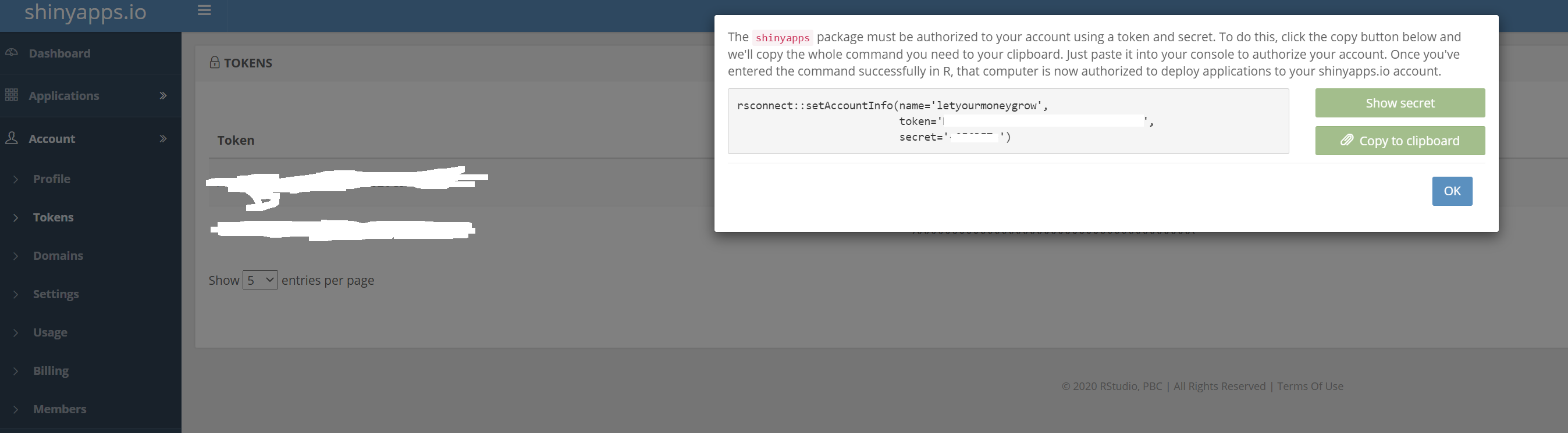
2) In your R-Studio set the working dir to app folder and then
> rsconnect::setAccountInfo(name="
> library(rsconnect)
> deployApp()
Preparing to deploy application...
Update application currently deployed at
https://letyourmoneygrow.shinyapps.io/shinyzinser/? [Y/n] y
DONE
Uploading bundle for application: 3357099...DONE
Deploying bundle: xxxxxxxx for application: yyyyyyy ...
Waiting for task: 835446185
building: Parsing manifest
building: Building image: zzzzzzz
building: Fetching packages
building: Installing packages
building: Installing files
building: Pushing image: xxxxxxx
deploying: Starting instances
rollforward: Activating new instances
unstaging: Stopping old instances
Application successfully deployed to https://letyourmoneygrow.shinyapps.io/shinyzinser/
3) If something goes wrong, shinyapp.io provide logs

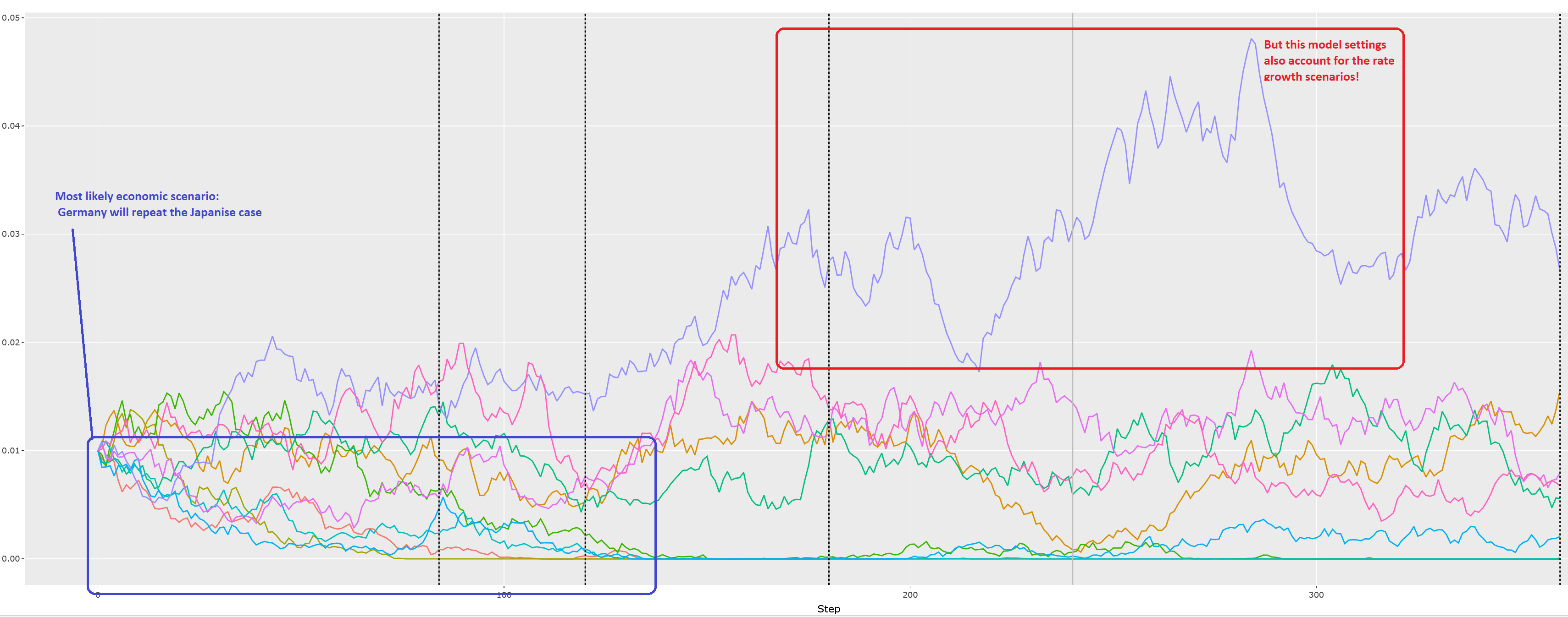
So far so good for technical part, but what about the business usage? Well, I gonna write a separate post on it and so far I would just like to mention that the simulation shows pretty distinctly: (sic! in my case) it is better to take the submortgages with a shorter duration and smaller rate!
Of course the simulation results depend on model assumptions very strongly. But the CIR model is pretty flexible, so I can (and of course do) generate very versatile economic scenarios.

Generally, I worked one day long on this app but it will likely save me about €30000 (over 30 years). A worthy investment, wouldn't you agree? If yes, do not hesitate to contact me!
FinViz - an advanced stock screener (both for technical and fundamental traders)