Numeracy for Traders - Lesson 2 - Exponentiation, polynomials, logarithms and the power of compound returns

After this lesson you will understand how to compute the compound return, discount factors and the CAGR (compound annual growth rate: nominal and inflation adjusted). You will also learn about the continuously compounded (exponential) interest and logarithmic returns. Finally, you will be able to calculate the effective rate of interest of a credit or of a savings scheme.

Albert Einstein used to say "Compound interest is the eighth wonder of the world. He who understands it, earns it ... he who doesn't ... pays it". Both parts of his sayings are true and very relevant for every investor. Manhattan was bought for 60 Gulden (about $30) in 1626, which is often considered to be a one of unfairest deals in the history. However, had Native Americans invested this money under 6% per annum (p.a.), they could have bought the Manhattan back with all current real estate four times! Interestingly, the Dow Jones Industrial Average (DJ30) grows approximately 6% p.a. in the long term. Though it is calculated only from 1986, the Amsterdam Stock Exchange was already founded in 1602, so making 6% CAGR since 1926 was, in principle, possible ... at least with a good risk management that would have recognized the tulip mania bubble.

Let us derive a formula to calculate the total yield by the interest rate $r$ after $n$ years. Let $K_0$ be your invested capital. After one year you get it back and, additionally, you get the interest, i.e. $r \cdot K_0$ . So in total you have $K_1 = K_0 + r K_0 = K_0(1+r)$ . Next year you invest $K_1 = K_0(1+r)$ and get in the end of the next year $K_1 + rK_1 = K_1(1+r) = K_0(1+r)(1+r) = K_0(1+r)^2$ .

Generally, after $n$ years your capital is $K_n = K_0 (1+r)^n$

But what if $n$ is a fractional number of years?! (In this case one usually writes $t$ instead of $n$ ). E.g. it is not uncommon to accrue the interest semi-annually or even quarterly. So in 3 months your capital is equal to $K_0 \sqrt[4]{1+r} = K_0 (1+r)^{\frac{1}{4}}$ and in 6 months it is $K_0 \sqrt{1+r} = K_0 (1+r)^{\frac{1}{2}}$
Note the following muliplicativity: $(\sqrt[4]{1+r})^4 = (\sqrt{1+r})^2 = (1+r)$ that also holds true for a general case

$K_t = K_0(1+r)^t$

There is still a nuance how to calculate the year fraction $t$ . The least time span for which the interest is accrued is a day. You likely know that there are overnight rates but there are no "intraday rates" (or at least they are not a common financial practice). But the approaches to convert the number of days in a year fraction (so-called day count conventions) and the ways to treat bank holidays (business day conventions) vary, although the difference under the bottom line is usually negligible. In our example we will use the simplest day count convention 30/360 (assume that there are 30 days in each month) and completely ignore the bank holidays (note that holidays affect only the date on which the accrued interest is booked to you account, but the interest is accrued on all days - whether working or holidays).

Besides the formula $K_0(1+r)^t$ - which was relatively hard to calculate for a general $t$ without a computer (try to compute it manually for, say, $r=6\%$ and $t=0.25$ ) - there is another common approach. If the interest is accrued semi-annually, for one year we calculate $(1+\frac{r}{2})^2$ and for a quarterly accruement we calculate $(1+\frac{r}{4})^4$ . Though we lose multiplicativity since $(1+\frac{r}{n})^n \ne (1+r)$ unless $r = 0$ , this approach is much more easy for the manual computation (remember, interest rates exist much longer than the computers and calculators). Moreover, there is an interesting observation: if we let $n \to 0$ we obtain

$\lim_{n \to 0}(1+\frac{r}{n})^n = \exp(r)$ or for a general time of investment $t$ : $K_t = K_0 \exp(rt)$

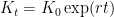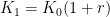
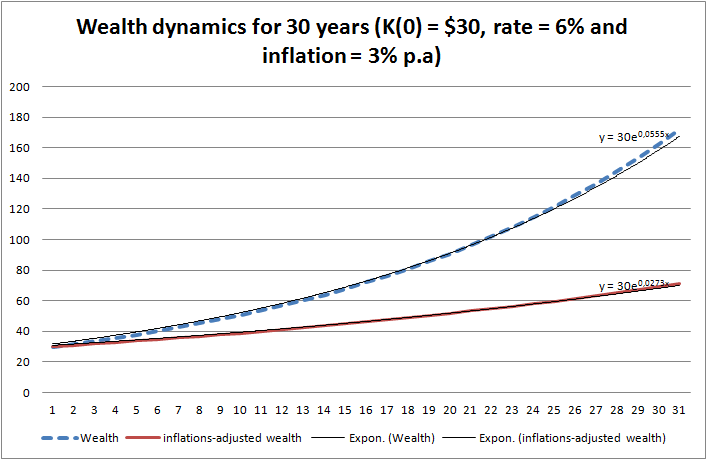
Let us compute the wealth dynamics for the first thirty years under assumption that the Native Americans would put $K_0 = \$30$ under 6% p.a.

wealth dynamics - Rate per annum vs exponential continuously compounded rate You see that in 30 years they would get almost the sixfold of the initial capital! But the same is true for a credit: if one borrows $30 and has to pay them back in 30 years, one will pay back $172.30! Think about it every time you take a loan!
But for the most of people it is difficult to perceive the exponential growth. Such growth does take place in the nature (population growth, powder explosion) but we hardly observe it directly. What we do observe since the stone-age era is a linear function (motion with a constant speed) and a quadratic function (motion with acceleration). But look how the exponential function beats them both over a long term (in this example 300 years)! That's why always calculate your loan costs, don't just rely on your gut feelings, they may let you down in this case!

exponential function vs. linear vs. quadratic over the period of 300 years Let's come back to the interest, compounded according to $\exp{(rt)}$ You see from the charts that it brings somewhat more yield than $(1+r)^t$ (on both charts the exponent is somewhat less than 0.06). This means that the more frequently the interest is compounded the better is for you (of course, if you deposit money). You also see that an exponential trend fit is nearly perfect, so you can always numerically switch from continuous compounding $\exp{(rt)}$ to the "normal" compounding $(1+r)^t$ and vice versa.
In practice there is virtually no continuously compounded returns but they are ubiquitous in the academic literature and they are very important in order to understand some principle concepts: first of all you readily see that the wealth grows exponentially.

The logarithm is the inverse of the exponential function and in case of continuously compounded rates it is especially easy to calculate the (annualized) return: $\text{CAGR}_t = \frac{\ln{K_t/K_0}}{t} = \frac{\ln{(\exp{(rt)})}}{t} = rt/t = r$
It is also common in academic literature to consider the logarithmic returns: $R^{\text{log}}_t = \log\left( \frac{K_t}{K_0} \right)$

However, since in practice they deal with "normal" compounding, the formula for the annualized return looks a little bit more complicated.
It holds $K_t = K_0(1+r)^t$ thus $\ln(\frac{K_t}{K_0}) = t\ln(1+r)$ and finally

$r = \exp{\left(\ln\left(\frac{K_t}{K_0}\right)/t\right)} - 1$

If you have an interest rate, you can also calculate the discount factors. For the continuous rates these are $\exp{(-rt)}$ and for the "normal" rates they are $\frac{1}{(1+r)^t} = (1+r)^{-t}$

The inflation is, in a sense, a discount factor. If the inflation rate is $i$ , so the formula for the dynamics of the inflation-adjusted wealth is $K^{\text{adj}}_t = K_0 \frac{(1+r)^t}{(1+i)^t}$

Wealth dynamics with and without inflation If we consider the inflation $i=3\%$ by the (nominal) annual growth rate of $r=6\%$ , we get the inflation-adjusted annual growth rate of $2.91\%$ (check it)! So you see that 1% of inflation decreases your wealth more than 1% of the growth rate increases it!

Finally, let us consider the loans and saving plans.
In case of a saving plan one invests (usually monthly) a fixed amount in an ETF. Contrary to the bank deposits, the returns on ETFs are random but for the calculation of the growth rate it doesn't matter much.
Assume that you invest monthly a fixed account $P$ and let $W_n$ be the total value of your savings after $n$ months. Then you have to solve the following equation

$P(1+r/12)^{n/12} + P(1+r/12)^{(n-1)/12} + ... + P(1+r/12) = W_n$

Note that for simplicity we assumed the integer number of months and simply divided the (implied) rate $r$ by 12. As you already know, it is not 100% precise but will do for the practical purposes if $r$ is relatively small (and normally it is).
This equation is a polynomial and if $n > 4$ then there is no closed-form solution. However, the result can easily be found iteratively, e.g. by means of the Excel Solver.

Analogously if you get a loan with a notional amount $K$ and pay a month installment $P$ you have to solve

$\frac{P}{(1+r/12)^{n/12}} + \frac{P}{(1+r/12)^{(n-1)/12}}+ ... + \frac{P}{(1+r/12)}= K$

Note that the monthly installment can be decomposed to the interest you pay to the bank and the debt redemption. The former is bad (it is what the bank earns on you) and the latter is good. We will not explain this decomposition in detail but you can understand it from the Excel sheet, in which we calculated all our examples.

Like this post and wanna learn more? Have a look at Knowledge rather than Hope: A Book for Retail Investors and Mathematical Finance Students

FinViz - an advanced stock screener (both for technical and fundamental traders)

Share this: