Perfect diversification means no asset can be dropped from (rather than added to) a portfolio

A common belief: adding extra asset to a portfolio will automatically reduce the portfolio risk. We provide a counter-example resorting only to the simplest algebra and explain why this erroneous belief is so common.

To diversify a portfolio in order to avoid severe losses in such cases as Enron scandal or Dieselgate is generally a very good idea. But still it is not always efficient. E.g. Volkwagen was the number one in automotive industry before the Dieselgate. Yet those, who did not just "bet on the leader" but broadly invested in automotive, have all the same experienced severe losses, since the scandal hurt the whole branch. Moreover, it is not uncommon to strictly limit the portfolio weight of a single stock but to tolerate significantly higher branch weight. Respectively, such "diversified" portfolios could have been hurt even stronger than those, which contained just a (strictly limited) position in Volkwagen.

Another motivation to diversify is to reduce the "natural" portfolio volatility, which is due to the market noise.

volatitily as a risk measure

You may probably doubt that the volatility is an appropriate measure of risk. Well, as any other risk measure it is not perfect but is also not as bad as it is sometimes criticized. Have a look at our short video tutorial!

[collapse]

But in context of this purpose adding an extra asset sometimes means more volatility, not less! How can it be?!
As I studied Quantitative Finance at the University of Ulm, a professor started the lecture about the diversification with a following example: assume there are two stocks, both with the expected return $r$ and the volatility $\sigma$ . Let their correlation coefficient be $\rho$ . Since the expectation is additive even for dependent random variables, the diversification will not affect the expected return. But does it make sense to diversify in order to reduce the portfolio variance?! To answer this question, put the wealth fraction $u$ in the first stock (respectively, $(1-u)$ in the second stock) and consider the portfolio variance, which is equal to $u^2 \sigma^2 + (1-u)^2 \sigma^2 + 2u(1-u) \rho \sigma^2 = \sigma^2(u^2 + 1 - 2u + u^2 + 2u\rho - 2u^2\rho)$
Further $2u^2 + 1 - 2u + 2u\rho - 2u^2\rho = 2u(u-1)(1-\rho) + 1$
Since $0 \le u \le 1$ and $-1 \le \rho \le 1$ , $2u(u-1)(1-\rho)$ is non-positive. In particular, it is equal to zero if $\rho=1$ , i.e. in case of the perfect positive correlation the diversification does not reduce the portfolio variance but otherwise it does!

Of course the assumption of both equal variance and expected return is somewhat restrictive. However, not too far from reality, especially if we consider the stocks from the same branch and country, the returns and volatilities will likely be similar. However, don't forget that we proved the statement only for the case of two stocks! But in case of three and more assets it may be not true anymore (unless we are allowed to sell short)!
Indeed, assume we have three assets, again with the same expected returns $r$ and volatilities $\sigma$ . But let the first and the second asset be uncorrelated, whereas let the correlation between the first and the third (as well as between the second and the third) asset be $\rho>0$ . Then the total portfolio variance is equal to
$\sigma^2[u_1^2 + u_2^2 + 2\rho u_1 (1 - u_1 - u_2) + 2 \rho u_2 (1 - u_1 - u_2) + (1 - u_1 - u_2)^2] \\ = \sigma^2[u_1^2 + u_2^2 +2\rho u_1 + 2\rho u_2 - 2\rho u_1^2 - 4\rho u_1 u_2 - 2 \rho u_2^2 + (1 - u_1 - u_2)^2] \\= \sigma^2[ u_1^2 + u_2^2 + 2\rho(u_1 + u_2)(1-u_1 - u_2) + (1 - u_1 - u_2)^2]$
Since we don't allow short selling, it holds that $u_1 + u_2 \le 1.0$ .
Since the 1st and the 2nd stocks are identical in the sense of their volatilities and correlations, the solution that minimizes the portfolio variance should be symmetric, i.e $u_1 = u_2$ . But of course it may (and it does) depend on $\rho$ .

We could have found a solutions by means of calculus but since we promised only a simple algebra, we find it numerically by means of the following R-code:

rho=seq(from=0.0, to=1.0, by=0.01)
u = seq(from=0.0, to=0.5, by=0.01)
vola = array(dim=101*51)
uArr = array(dim=101*51)
rhoArr = array(dim=101*51)
idx = array(0.0, dim=101)
j=0
for(i in 1:100)
{
 volaMin = 1000.0
 for(k in 1:51) 
 {
 j = j+1;
 uArr[j] = u[k];
 rhoArr[j] = rho[i]
 vola[j] = 2*u[k]*u[k] + 2*rho[i]*2*u[k]*(1-2*u[k]) + (1-2*u[k])*(1-2*u[k])
 if(volaMin>vola[j]) 
 {
 idx[i] = j
 volaMin = vola[j]
 } 
 }
} 
idx1 = which(rhoArr==0.2)
idx2 = which(rhoArr==0.5)
idx3 = which(rhoArr==0.6)
library(scatterplot3d)
s3d <- scatterplot3d(uArr,rhoArr, vola, main="Portfolio Variance - by rho={0.2, 0.5, 0.6} an min. curve (yellow)")
s3d$points(uArr[idx1], rhoArr[idx1], vola[idx1], type="o", col="red", lwd=2)
s3d$points(uArr[idx2], rhoArr[idx2], vola[idx2], type="o", col="blue", lwd=2)
s3d$points(uArr[idx3], rhoArr[idx3], vola[idx3], type="o", col="green", lwd=2)
s3d$points(uArr[idx], rhoArr[idx], vola[idx], type="h", col="yellow", lwd=1)

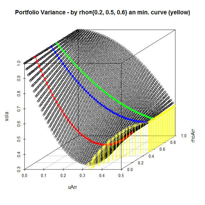Portfolio Variance depending on u1=u2 and rho One can readily see that by $\rho < 0.5$ it still does make sense to diversify with a 3rd stock but by $\rho \ge 0.5$ not anymore!
In other words: in this case adding the third asset to the portfolio means making it more risky!

upper bound of rho

We plotted $\rho$ from 0.0 to 1.0. But its real upper bound is lower. In particular, $\rho=1.0$ would have meant that the 3rd stock perfectly correlates with both the 1st and the 2nd but then the 1st and the 2nd stocks cannot be independent! In case of a normally distributed returns we can estimate the upper bound of the $\rho$ analyzing the Cholesky decomposition of the correlation matrix. In a more general case the problem is much more challenging. Fortunately, we do not necessarily need to solve it for our practical purpose.

[collapse]

But do such cases take place in practice? Well, occasionally, but they do!
After some trial and errors (looking for a proper loopback period) I constructed such case with the stocks of BMW, SAP and Beiersdorf.
The covariance matrix of their daily returns is as follows.

	BEI.DE	SAP.DE	BMW.DE
BEI.DE	0.00016999	0.00011504	0.00014119
SAP.DE	0.00011504	0.00018701	0.00015599
BMW.DE	0.00014119	0.00015599	0.00031560

The variance and covariances of the BMW stock are so big that the optimal solution is not to include this stock in portfolio at all. Moreover, in this case BMW also has a negative expected return! So there is even no trade-off between the expected return and the volatility of the portfolio.

Mean daily returns
BEI.DE	SAP.DE	BMW.DE
7.892253e-05	1.148840e-04	-1.558986e-04

As usual, we provide R-code to reproduce the results.
It uses library quadprog to find a optimal solution with no leverage and no short selling. Look at this excellent post if you what to learn more about quadprog usage for portfolio optimization.

library(quantmod)
stocks = c("BEI.DE", "SAP.DE", "BMW.DE")
getSymbols(stocks, from="2014-01-01", to="2016-05-01") 
#from and to define the loopback period

bmw = as.vector(BMW.DE[,6])
LEN = length(bmw)
bmwRets = diff(bmw) / bmw[2:LEN] 
bei = as.vector(BEI.DE[,6])
beiRets = diff(bei) / bei[2:LEN] 
sap = as.vector(SAP.DE[,6])
sapRets = diff(sap) / sap[2:LEN] 
dataFrame = cbind(beiRets,sapRets,bmwRets)
cor(dataFrame)
S = cov(dataFrame)
mu = colMeans(dataFrame)

library(quadprog)
dvec=c(0,0,0) #just minimize the portfolio variance
Amat <- cbind(1, diag(nrow(S)))
bvec <- c(1, rep(0, nrow(S)))
meq <- 1
qp <- solve.QP(S, dvec, Amat, bvec, meq)
qp$solution

SUPPLEMENT: letYourMoneyGrow.com is very grateful to Alen Horvat, who carefully read this post, corrected some errors and wrote a more technical follow-up.