Seeking Alpha and finding nonsense - never trust CAPM and linear regression blindly

I show by the example of my portfolio "somewhat better than DUCKS" that CAPM alpha is a very non-robust measure of performance as well as that linear regression on an index should be considered very critically.

Recently, one of my facebook contacts has meant that my portfolio "Somewhat better than DUCKS" repeats the DAX with a beta but without alpha. He even did not make an effort to calculate the linear regression before making this statement. However, even if he did, the results would not be comprehensive.

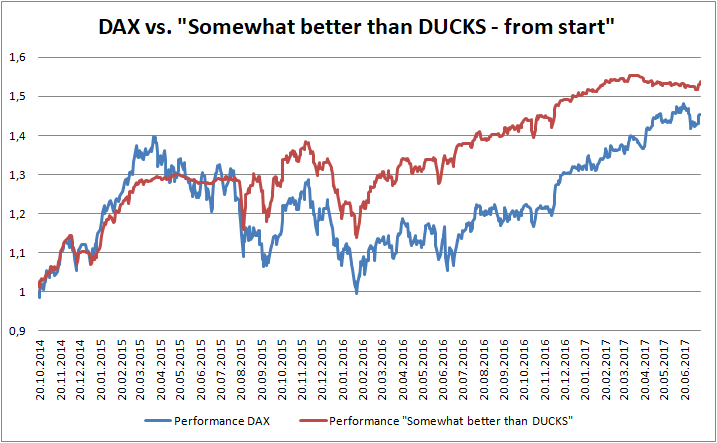
The chart clearly shows that - measuring from the start - my portfolio outperforms the DAX. And if we make a linear regression of portfolio returns on the DAX returns, we become $r_{port} = 0.0004647 + 0.2968241 r_{DAX}$ (we assume riskfree rate is zero, which is the case in Germany, indeed it is even negative due to Strafzins). A daily alpha of 0.0004647 is not small: annualized it means $(1+0.0004647) ^{ 242 \text{ (trading days)}} = 0.119$ , i.e. 11.9% of extra return!

However, the lower and upper bounds are as follows:

Confidence interval	2.5 %	97.5 %
(Intercept) ( $\alpha$ )	-0.0000326981	0.0009621773
as.vector(copdat$RetsDAX) ( $\beta$ )	0.2579411899	0.3357070687

Since the 95%-confidence interval covers zero, there is, strictly speaking, no statistically significant alpha. Had we taken e.g. 90%-confidence interval, the alpha would be significant, but ok, 95% and 99% are the most common critical levels, so we shall not arbitrarily manipulate them.

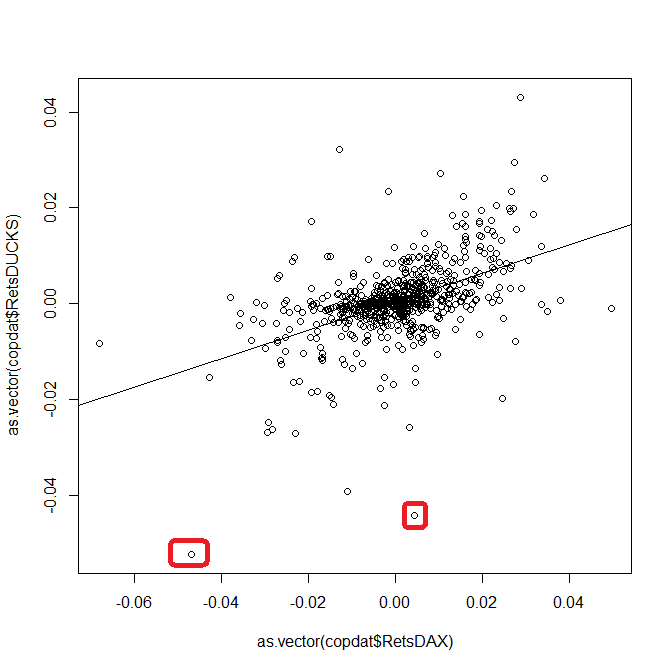
However, let us see what happens if we remove just two largest outliers (they are marked with red).
In this case the alpha is equal to 0.0005959 and is significant at 95% confidence level since the confidence interval is:

Confidence interval	2.5 %	97.5 %
(Intercept) ( $\alpha$ )	0.0001287635	0.001062976
as.vector(copdat$RetsDAX) ( $\beta$ )	0.2447805626	0.318531328

The regression plot looks in this case as follows:

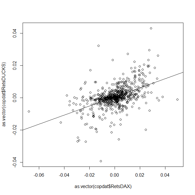
As you can readily see, there is no big difference with a previous plot but the conclusion is principally different!

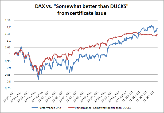
Finally, if we consider the performance of my fund vs. DAX since the date my fund become investable, we see that though I continued to outperform the DAX, for the latest months it is not the case (it will likely be the again the case soon but so far the DAX overtakes me on absolute performance basis).

Interestingly, in this case the fitted intercept is equal to 0.0001702. Although the lower bound of the 95% confidence interval is -0.0003204815 (which again means no statistical significance), a naive interpretation of the linear regression would imply that I have a positive alpha also in this case.
Makes of course little sense, since it is the terminal wealth what matters.

Fortunately, there is a simple explanation behind all these "paradoxes".
First of all, I have significantly beaten the DAX twice: first time when I anticipated the drop in the middle of 2015 and second time as I optimally structured my portfolio before the Brexit. On the other hand I lost to DAX during recent month since I followed "sell in May and go away" but in 2017 the stocks did not follow this saying.
In particular, it means that several days may be decisive and the returns on them may be far from being normally distributed. It is not yet an invalidation of the least squares, however, it may drastically distort the confidence intervals.

That's why: never substitute common sense with a quantitative analysis, esp. such a simplified approach as linear regression. In particular, it should catch your eye that the $\beta$ is only about 32% (the correlation of daily returns is ca. 63%, which is also not that much). The reason behind it is that I sometimes go short and DAX and also trade some commodities. It is immediately clear if you browse the history of trades but no linear regression will show it!

Supplement:

Source data and R-code:

#first copy the data to clipboard from respective .txt file
copdat <- read.delim("clipboard")
plot(as.vector(copdat$RetsDAX), as.vector(copdat$RetsDUCKS))
linMod = lm(as.vector(copdat$RetsDUCKS) ~ as.vector(copdat$RetsDAX))
linMod
abline(linMod)
confint(linMod)
cor(as.vector(copdat$RetsDUCKS), as.vector(copdat$RetsDAX))