PCA, Autoencoders and the Feasibility of Stockpicking

The idea that the stock picking makes less and less sense since the markets are more and more driven by the macroeconomic factors is quite popular.
Especially right now, as the markets are falling (like on todays FEd decision to increase the rates), this idea may seem to be plausible. However, we show that in the long term the stocks do show enough of individuality.

To demonstrate our statement we use the historical returns of all DowJones stocks from 2010. Why from 2010? Well, because we do not argue that in crisis (or even a strong market correction) they generally fall together.
But let us have a look how it was during the bool market.

To get the data from Yahoo.Finance run the following R-code (if Yahoo.Finance again ceases to work, contact us and mention that you need DJ30_dailyReturns_from2010 dataset; unfortunately we cannot publicly re-distribute Yahoo's data).

library(quantmod)
#
DJ30tickers = c("MMM", "AXP", "AAPL", "BA", "CAT", "CVX", "CSCO", "KO", "DIS", "DWDP", "XOM",
"GS", "HD", "IBM", "INTC", "JNJ", "JPM", "MCD", "MRK", "MSFT", "NKE",
"PFE", "PG", "TRV", "UTX", "UNH", "VZ", "V", "WMT", "WBA")
#
DJ30histDat = list()
DJ30histOHLC = list()
N = length(DJ30tickers)
for(j in 1:N)
{
  foo = getSymbols(DJ30tickers[j], auto.assign=FALSE, from="2010-01-01", to="2018-12-18")
  goo = xts(foo[,6], order.by=index(foo)) #adjusted prices
  boo = xts(foo[,1:4], order.by=index(foo)) #OHLC
  DJ30histDat[[DJ30tickers[j]]] = goo
  DJ30histOHLC[[DJ30tickers[j]]] = boo 
}
for(j in 1:N) 
    print(length(DJ30histDat[[DJ30tickers[j]]])) #just test that they all have the same length

L=length(DJ30histDat[[DJ30tickers[1]]])
rets = array(0.0, dim=c(L, N))
for(j in 1:N)
{
    rets[,j] = as.numeric(dailyReturn(DJ30histDat[[DJ30tickers[j]]]))
}
#
retsDF = as.data.frame(rets, row.names=index(foo))
colnames(retsDF) = DJ30tickers

First of all let us have a look at the (nicely visualized) correlation matrix of returns.

library("ggcorrplot")
ggcorrplot(cor(retsDF), method = "circle", lab=TRUE)

Although all correlations are positive, their typical value lays between 0.3 and 0.6, which is not too big.

Let us now check whether we can reduce the dimensionality by means of the principle component analysis (i.e. switch from 30 stocks to a couple of factor variables).

plot(prcomp(retsDF)$sdev)

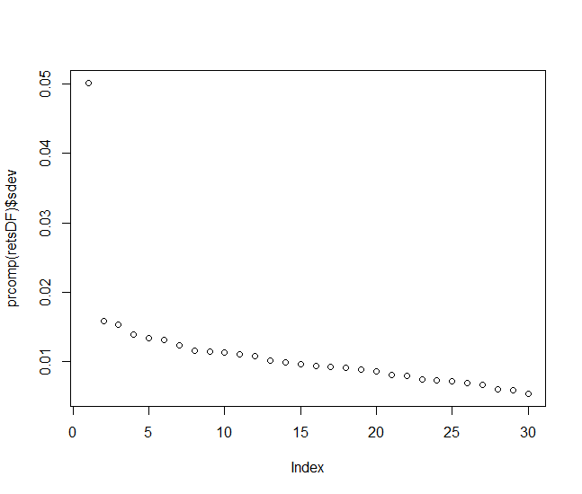
You see that although there is one dominating factor (which obviously can be interpreted the macroeconomy), its domination is not overwhelming. Moreover, the variance of other factors decays slowly, which means that even several factors (e.g. one factor for each industry sector) would hardly be sufficient to model the market without a significant loss of information.

As the last step (which is rather superfluous for the practical goals but good for educational purposes) let us try to do the same with a neural network autoencoder.
Finally, the principle component analysis can only catch linear relations, whereas a neural network can (theoretically) catch pretty everything.

library(keras)
b = floor(0.8*L)
x_train = rets[1:b,]
x_test = rets[(b+1):L,]
y_train = x_train
y_test = x_test
##############################################
model <- keras_model_sequential() 
model %>% 
  layer_dense(units = 30, activation = 'linear', input_shape = c(30)) %>% 
summary(model)
model %>% compile(
  loss = 'mean_squared_error',
  optimizer = optimizer_adam(),
  metrics = c('accuracy')
)
history <- model %>% fit(
  x_train, y_train, 
  epochs = 200, batch_size = 100, 
  validation_split = 0.2
)
plot(history)
model %>% evaluate(x_test, y_test)

We start with a primitiv neural network, containing 30 units and activated by a linear function (essentially this network is expected to learn to apply the Identity transform, or in simple words to do nothing (have a look at get_weights(model))).

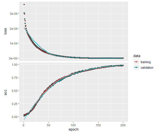
Note that if you replace activation = 'linear' with activation = 'sigmoid',, the model calibration will generally fail!
. Why is it so? Well, most likely because the sigmoid is a strictly positive function... but why it is not shifted by b[ias] coefficient?... Anyway, put e.g. the tanh instead and everything will be ok again.

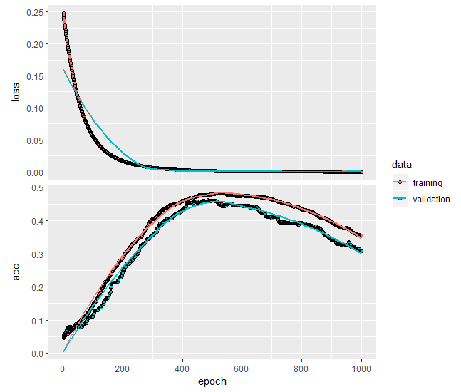
modelAccuracy = array(0.0, dim=30)
for(aeUnits in 1:30)
{
model <- keras_model_sequential() 
model %>% 
  layer_dense(units = 30, activation = 'tanh', input_shape = c(30)) %>% 
  layer_dense(units = aeUnits, activation = 'tanh') %>% 
  layer_dense(units = 30, activation = 'tanh') %>% 
summary(model)
model %>% compile(
  loss = 'mean_squared_error',
  optimizer = optimizer_adam(),
  metrics = c('accuracy')
)
history <- model %>% fit(
  x_train, y_train, 
  epochs = 200, batch_size = 100, 
  validation_split = 0.2
)
  plot(history)
  model %>% evaluate(x_test, y_test)
  modelAccuracy[aeUnits] = as.numeric((model %>% evaluate(x_test, y_test))$acc)
}
plot(modelAccuracy, main="Model Accuracy", xlab="AE-units in hidden layer")

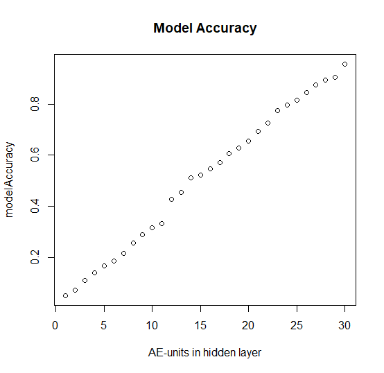
Interestingly, the model accuracy grows almost perfectly linearly with the number of the neurons in hidden layer in the middle.
This means that the autoencoder fails to compress the Information... but I expected that it would do at least as good as the PCA (in which the first component clearly dominates at the chart). We, however, postpone the discussion of this topic for the future posts, stay tuned!