Optimal Number of Trades: better less but better

A very important question, which every trader or investor encounters is how many trades to commit or how many stocks to hold in portfolio. Whereas the law of the large numbers readily gives a [naive] answer "the more the better", in practice the answer is often better less but better.

In order to be a profitable trader it is necessarily to have a positive expectation of trades. For the sake of simplicity let us assume that a trader closes his position as the profit or loss reaches 10% (or 20% for highly volatile stocks). 10% and 20% are not arbitrary numbers: look at the boxplot of quarterly returns for the following stocks and you will readily see that a typical stock quarterly return (i.e. what resides within the boxes) is quite in range of [-20%, +20%]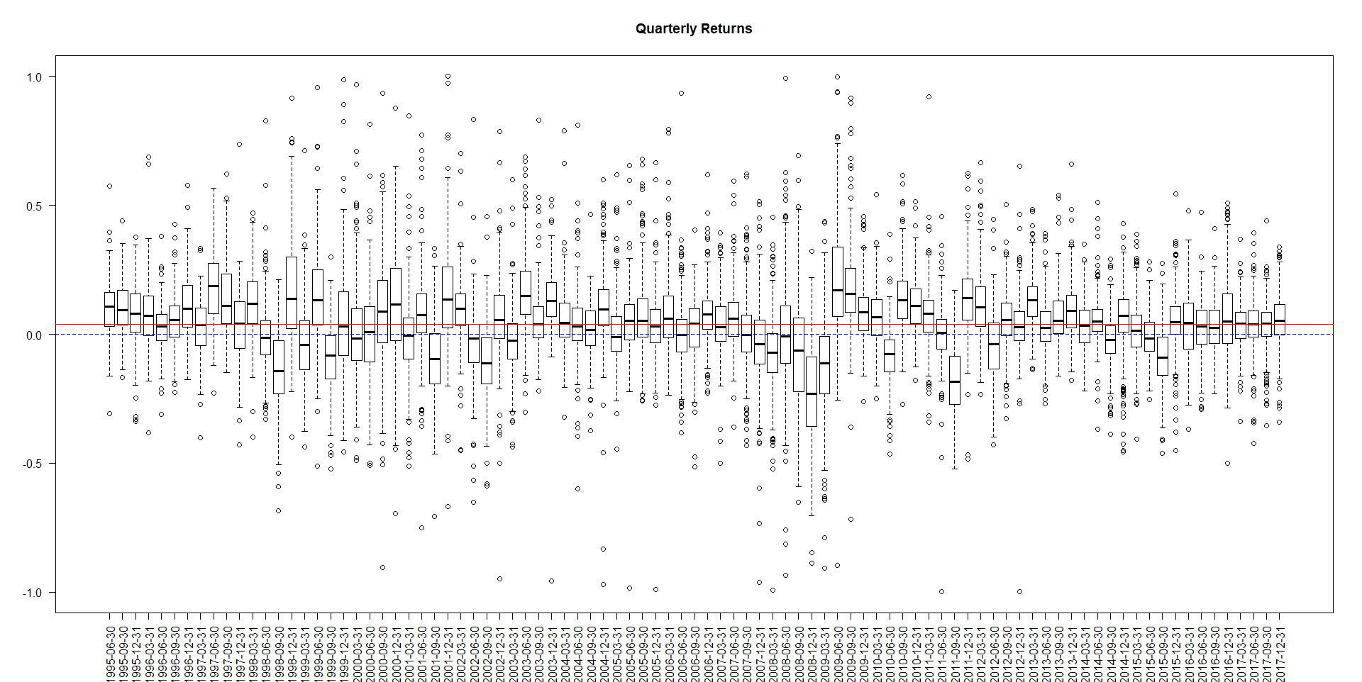

The next question is which winning percentage is realistic. Well, previously we have analyzed the performance of two star traders: Einstein and HBecker. Einstein has "merely" 56.77% of profitable trades, whereas HBecker has 75.87% (which is a really a great hit rate and hardly can be exceeded, at least we do not know anybody who has a better rate).

So let us start with the winning percentage of 55%. Obviously, this is a relatively small rate thus one needs a sufficient number of trades (or stocks in portfolio) to gain from it with sufficiently high probability. But trading and picking the stocks is a pretty time-consuming task, if done properly. So assuming maximum 100 trades or stocks in portfolio is not implausible. Indeed, we were talking about quarterly returns, so 100 trades within 3 months is pretty a lot.
As to 100 stocks in portfolio, it is not too hard to find 100 good stocks but is much harder to find 100 good and loosely correlated stocks. The latter is crucial, as we showed before, adding a highly correlated stock to a portfolio can worsen the diversification!
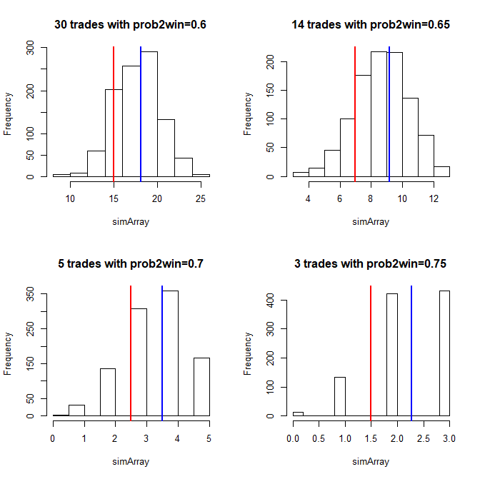
For 100 uncorrelated stocks or trades the probability to make a loss is just 13.46% (check it in R with pbinom(49, 100, 0.55)). But, as we have just said, 100 uncorrelated stocks or trades may be a challenge. So let us consider the hit rates of 60%, 65%, 70% and 75% and calculate the required number of trades in order to have approximately the same probability of loss. These quantities are 29, 13, 5 and 3 (you easily check it with the following R script).

probs = c(0.55, 0.6, 0.65, 0.7, 0.75)
N_TRADES = c(100, 29, 13, 5, 3)
for(j in 1:length(probs)) 
{
    half = N_TRADES[j] / 2
    if(!(N_TRADES[j] %% 2))
        half = (N_TRADES[j] / 2) - 1  

    print(round(pbinom(half, N_TRADES[j], probs[j]),4))
}

To find 14 virtually uncorrelated stocks is a realistic task, which gets even easier if we consider not only stocks but also bonds, commodities and currencies (no cryptocurrencies, please :))

Taking the probability of loss as a starting point is not an implausible idea, since (esp. for the novices) an important goal by trading is not to lose money. However, this single number does not give us a complete overview, so let us have a look at the PnL distributions (red line means breakeven border, blue line is the expected number of winning trades).

par(mfrow=c(2,2))
N_SIM = 1000
for(j in 2:5)
{
    simArray = array(0, dim=N_SIM)
    for(k in 1:N_SIM)
    {
        simArray[k] = sum(rbinom(N_TRADES[j], 1, probs[j]))
    }
    hist(simArray, main=paste0(N_TRADES[j], " trades with prob2win=",probs[j]))
    abline(v=N_TRADES[j]/2, col="red", lwd=2)
    abline(v=mean(simArray), col="blue", lwd=2)
}

As you can see, the expected number of profitable trades grows with the probability to win(surprise, surprise!). However, the tails (i.e. the probabilities of severe losses) also do. So let us simulate our terminal wealth.

N_QUARTERS = 20 #5 years
N_SIM = 1000
PnL = 0.2 #20%
wealthArray = array(1.0, dim=c(N_QUARTERS+1, N_SIM, 4))
for(j in 2:5)
{
    for(qu in 1:N_QUARTERS)
    {
      for(si in 1:N_SIM)
      {
         outcome = rbinom(N_TRADES[j], 1, probs[j])
         outcome[which(outcome==0)] = -1
         wealthArray[qu+1, si, j-1] = wealthArray[qu, si, j-1] * (1 + PnL*mean(outcome))
      }
    }
}
plot(density((wealthArray[N_QUARTERS+1,,1])), xlim=c(min(wealthArray), max(wealthArray)), main="Terminal wealth densities")
lines(density((wealthArray[N_QUARTERS+1,,2])), col="red")
lines(density((wealthArray[N_QUARTERS+1,,3])), col="blue")
lines(density((wealthArray[N_QUARTERS+1,,4])), col="green")
abline(v=1.0, col="grey", lty=2)
#the same to see the risk tails
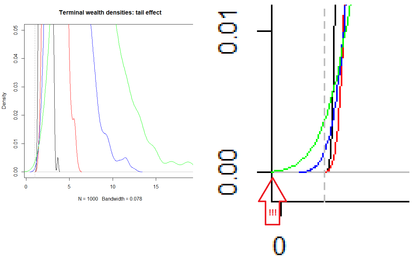
plot(density((wealthArray[N_QUARTERS+1,,1])), xlim=c(0.8*min(wealthArray), max(wealthArray)), ylim=c(0, 0.05), main="Terminal wealth densities: tail effect")
lines(density((wealthArray[N_QUARTERS+1,,2])), col="red")
lines(density((wealthArray[N_QUARTERS+1,,3])), col="blue")
lines(density((wealthArray[N_QUARTERS+1,,4])), col="green")
abline(v=1.0, col="grey", lty=2)

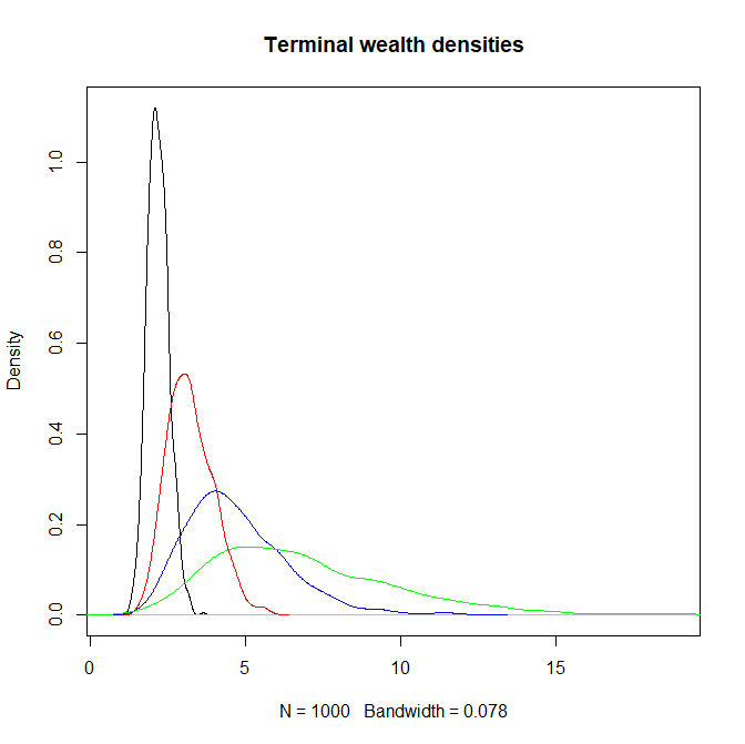
As to me, I would prefer the red variant (e.g. 13 trades with 65% hit rate).
As you can see, it is the least risky (has the lightest tail) and brings a sufficient expected gain (better than the black one with 29 trades and 60% hit rate). Although the blue and the green bring on average even more, they have too heavy tails, which may be unacceptable for a risk-averse investor.

Note, however, that the green tail does not reach zero (i.e. total loss), it is just an artifact of the kernel smoothing, which is used to draw the density function. The maximum loss was -35% in this simulation... which might also be painful.
Of course this (as well as other simulation results) depend on the choice of N_QUARTERS and PnL parameters, so try with different constellations of them.